This might be helpful. Similar to pytest, but to automatically compile the notebooks and relay any errors.

https://github.com/ReviewNB/treon?utm_campaign=Data_Elixir&utm_medium=email&utm_source=Data_Elixir_229

On xr_corr, need to suppress warnings for NaNs. This is done for compute functions, but I want to get the issue at the source. Easy fix when I have time.

@aaronspring, it seems like the dimension names expected for climpred are getting confusing once again. To align all products (control, initialized ensemble, observations, references), we have to rename our time dimension to initialization. This clearly doesn't make sense since the LENS for instance is defined by not being initialized. Further, not every single time step of that dimension is necessarily an initialization point.

Also, our perfect_model vs. reference_ensemble setup has begun to diverge with this. Currently, the perfect_model notebook expects a 'time' dimension for the control run for things like DPP and compute_skill. The reference_ensemble expects 'initialization' dimension and this has been incorporated into the relative entropy function for a LENS-like setup.

I suggest the following (hopefully final) changes for more clarity for us and future users:

• Go back to using time as the main dimension for any of these simulations. This makes sense, since it's the default dimension name that comes out of most simulations. This doesn't imply that every time step is an initialization and doesn't force us to rename time to initialization for a control run or uninitialized ensemble, which makes no sense.
• Remove initialization entirely. This is a long word and doesn't make sense for many cases.
• Use lead as the new dimension that is returned from many of our functions. Although lead time makes more sense, this requires annoying dictionary indexing to deal with since there is a space in it. lead is a unique dimension that shouldn't exist in any simulations and would only come out of our functions. It also makes more sense than time which we are currently using for lead time, which conflicts with the standard CF conventions for simulations.

This I think would help us avoid all confusion in the future. I am happy to do all the renaming and then we stick to this language for the object-oriented implementation.

https://app.codacy.com/project/ESMValGroup/ESMValTool/dashboard

Maybe can add this app to our repo.

This package looked interesting so I started playing with the DPLE_hindcast_prediction notebook, and I just wanted to leave a few comments.

1. CESM DPLE; I know about CESM, but I'm unfamiliar with DPLE and it wasn't until midway I encountered the title Decadal Prediction Large Ensemble. So I think it might be good to define the acronyms on the first encounter, e.g. What are we comparing the actual Decadal Prediction Large Ensemble (DPLE) to?

2. The name of the notebook doesn't match the first markdown cell: DPLE_hindcast_prediction vs Reconstruction-based Prediction Demo which I thought to be slightly confusing.

3. I think because proplot is in its development stage, there were keywords that were changed (probably related to https://github.com/bradyrx/climpred/issues/88). One example:

f, ax = plot.subplots(axwidth=4, aspect=1, rightpanel=True)
TypeError: _subplots_kwargs() got an unexpected keyword argument 'rightpanel'

Anyways, I think this is a great effort; I'm still trying to grasp it all, but I would love to contribute eventually! (Maybe a quick start guide would be helpful too!)

Incorporate a function to compute mutual information

I think this package has moved very far away from my esmtools personal package of functions, which is a good thing. I will probably create my own mini package later that incorporates some random functions, especially visualization stuff, that I need.

That being said, we should start to rebrand it for its eventual release to the seasonal/decadal climate prediction community. Thus, do you have any ideas for renaming this package?

PEP8 suggests:

Python packages should also have short, all-lowercase names, although the use of underscores is discouraged.

Some ideas:

• climpred

• decpred -- although this isn't explicit to climate-related prediction

I want to distinguish that this is for climate prediction, and not just prediction, since that's a whole field of time series analysis.

Incorporate a function to compute relative entropy, per Kleeman et al. 2002 (https://journals.ametsoc.org/doi/abs/10.1175/1520-0469(2002)059%3C2057:MDPUUR%3E2.0.CO%3B2) and Branstator and Teng 2010 (https://journals.ametsoc.org/doi/abs/10.1175/2010JCLI3678.1)

@aaronspring, are you familiar with MurCSS? Looks like an MPI-related project.

https://github.com/illing2005/murcss
https://www-miklip.dkrz.de/about/murcss/

This does something similar to climpred but I don't think it has as many metrics, or advanced functions like relative entropy.

I split our persistence computations into compute_persistence (original) and compute_persistence_pm (your new addition) in b912731. We should discuss our thoughts here.

The new method is not totally clear to me, particularly for a "reference" ensemble. In a reference ensemble, the DP system is initialized from one realization of a reconstruction. So here, the persistence forecast should be done to the full reconstruction (but should be subset to the time period the DP system covers). This is because the reference simulation is a continuous simulation. Subsetting that would cause discontinuities in the dynamics and would not accurately represent a true persistence forecast (i.e., next year is forecast for this year's anomalies).

I think if you're bootstrapping and are spinning off lead-time comparisons from a control, you can use your method. This is because each "initialization" has a self-contained time series you can compute persistence over with its own dynamics. This wouldn't cause a jump in the time series like it would with a reference ensemble.

Thoughts?

ref:

def compute_persistence(ds, reference, nlags, metric='pearson_r', dim='time'):
    """
    Computes the skill of  a persistence forecast from a reference
    (e.g., hindcast/assimilation) or control run.
    This simply applies some metric on the input out to some lag. The user
    should avoid computing persistence with prebuilt ACF functions in e.g.,
    python, MATLAB, R as they tend to use FFT methods for speed but incorporate
    error due to this.
    Currently supported metrics for persistence:
    * pearson_r
    * rmse
    * mse
    * mae
    Reference:
    * Chapter 8 (Short-Term Climate Prediction) in
        Van den Dool, Huug. Empirical methods in short-term climate prediction.
        Oxford University Press, 2007.
    Args:
        ds (xarray object): The initialization years to get persistence from.
        reference (xarray object): The reference time series.
        nlags (int): Number of lags to compute persistence to.
        metric (str): Metric name to apply at each lag for the persistence
                      computation. Default: 'pearson_r'
        dim (str): Dimension over which to compute persistence forecast.
                   Default: 'ensemble'
    Returns:
        pers (xarray object): Results of persistence forecast with the input
                              metric applied.
    """
    _check_xarray(reference)
    metric = _get_metric_function(metric)
    if metric not in [_pearson_r, _rmse, _mse, _mae]:
        raise ValueError("""Please select between the following metrics:
            'pearson_r',
            'rmse',
            'mse',
            'mae'""")
    plag = []  # holds results of persistence for each lag
    inits = ds['initialization'].values
    reference = reference.isel({dim: slice(0, -nlags)})
    for lag in range(1, 1 + nlags):
        ref = reference.sel({dim: inits + lag})
        fct = reference.sel({dim: inits})
        ref[dim] = fct[dim]
        plag.append(metric(ref, fct, dim=dim))
    pers = xr.concat(plag, 'time')
    pers['time'] = np.arange(1, 1 + nlags)
    return pers

our package is designed for decadal predictions, but once we start using monthly or seasonal output, we might have to adapt:

• still everything consistent
• how is datetime index treated in compute functions
• persistence forecast to incorporate climatology
• how to normalize for PM

I think we should spend another PR on terminology. Maybe even create a markdown file on terminology and conventional use of certain terms.

I would like to change metrics to skill scores as defined in Jolliffe 2011. Ch.2.7 Accuracy, association and skill:

Skill scores are often in the form of an index that takes the value 1 for a perfect forecast and 0 for the reference forecast. Such an index can be constructed in the following way:

In this way I would create an rmse-ss which is like 1-nrmse. ACC is already a skill score. then the rmse, mse and mse would still remain as distance measures, but all the skill scores would be good if close to 1, 0 if as good as reference and negative if worse. This might make the use of my limit-flag only for distance-based metrics, but not the skill scores.

We need to spend some time cleaning up the prediction.py module to make it more clear and organized.

Some tasks:

• Keep all import statements at top of module
• Make internal functions clear. I.e., use prefix underscore notation for functions that are only used internally by the module and should not be used by the user (https://dbader.org/blog/meaning-of-underscores-in-python)
• Separate the code into blocks of relevant code. (See clear blocking here, use of underscore notation: https://github.com/lukelbd/proplot/blob/master/proplot/base.py)
• Ensure that all functions (particularly functions that users will use) have clear documentation with citations. Many have this, but some require it

Goes long the thinking of documentation in metadata.

I am unsure about the requirements: are you more familiar @bradyrx

• time first dimension
• time in seconds since??

What I want to do with saved skill netcdf files:

• look at in with ncview
• use with cdo (doesn’t work now)

automatically checks python syntax with black or yapf

A feature to add to the object-oriented PR. One might have various products with different time slices. For instance, the reconstruction could go from 1950-2018, the initialized ensemble 1960-2015, and some observations 1990-2017.

So the user isn't constantly slicing things, we can always align to the common period, i.e., 1990-2015 for the above example. I'll work on adding this when I have time.

@aaronspring, I think you should take on this next PR for a few more updates. I think we're in great shape following the most recent merge -- thanks for all the feedback.

What I think needs to be addressed:

• (highest priority) Consolidate the damped persistence forecast into a function called compute_damped_persistence and it should work for perfect-model or reference, similar to compute_persistence. I imagine the new _shift function would be included. Currently, there are four separate functions pertaining to damped persistence, which is too much.

• (medium priority) Remove everything under the "SAMPLE DATA" section. I don't like having extra dependencies we don't need (this involves BeautifulSoup). We can add to our setup.py file a package_data keyword so that users can opt to download our processed sample data with the package.

• ( low priority) Clean up the perfect-model prediction notebook to be more clear (see the DPLE hindcast notebook now). It would be nice to have a background on what perfect-model means, using the high-level functions, etc.

• Make sure to install something like flake8 or use your editor that does auto-PEP8. It's best we stay within these standards from every PR forward.

I think we can save the metrics updates for the next PR, unless you want to include it in this one. Basically, we should have a metrics.py submodule that is similar to xskillscore that has speedy metrics.

@aaronspring, wanted to move this to an issue thread so we don't forget about it. As mentioned in bradyrx/esmtools#16, we should find a better solution for the chunking definition than the following:

def chunking(ds, number_chunks=False, chunk_length=False, output=False, time_dim='year'):

I'm not sure what it is. Maybe it involves dictionaries or something, but there might be StackExchange solutions out there.

Currently, esmtools.vis.deseam is unnecessarily complex. Cartopy has a function called add_cyclic_point that will drastically simplify deseam.

https://www.metoffice.gov.uk/research/climate/seasonal-to-decadal/gpc-outlooks/user-guide/interpret-reliability

Those kind of plots would be great. Didn’t find a suitable package for that, for did I understand all the details.

My version of https://github.com/bradyrx/climpred/issues/46

So far I only bootstrapped the threshold of skill from an uninitialized ensemble. My persistence forecast and the signal was without any uncertainty.

I will implement a bootstrapping on those.

Expected result:
http://hdl.handle.net/21.11116/0000-0002-0A63-4 Fig. 4.7, but also applicable to maps.

I really like this function, especially as it works on multiple dimensions. However, it doesnt work on xr.Datasets. Do you see an easy fix for this?

My current workaround: .to_array() create variable...
esmtools.stats.xr_rm_poly(DPE.to_array().isel(variable=0),2, dim='ensemble')

Why am I raising this? To me this is of low priority, but in general we should opt for xr.Dataset and xr.DataArray compatibility. input-type=output-type

Write function to incorporate linear breakpoint fit for DPP (Seferian 2018)

CC @aaronspring, per our conversation today. I added a prediction submodule to the develop branch. Perhaps we should chat about what functions to add here, as I am new to decadal prediction metrics.

--process-dependency-links is required for installing climpred since xskillscore is not on PyPI. However, it will soon be deprecated and is clunky anyways. (See pypa/pip#4187)

We need to find another way to force an xskillscore install when users install climpred. Alternatively we could just rewrite the pearson_r and rmse functions in our metrics submodule (once we make it), although that feels like stealing.

would be great to have the co2flux (Lovenduski2007) decomposition included ,@bradyrx.

Basically this code
https://github.com/bradyrx/EBUS_BGC_Variability/blob/master/notebooks/CO2_Flux_Decomposition/co2_flux_decomposition.ipynb
into
https://github.com/bradyrx/esmtools/blob/develop/esmtools/carbon.py

Another decomposition which would not rely on Takahashi's empirical 0.0423 factor is described in https://www.biogeosciences.net/15/5315/2018/bg-15-5315-2018.html

@aaronspring, I just found out about the wiki feature on github repositories. Let's develop our documentation there for now. It will be nice to get all of the content there, and then we can migrate to a sphinx-style website eventually.

You'll see a tab at the top of the repo labeled "wiki" (https://github.com/bradyrx/climpred/wiki) and you should be able to edit it since you're a collaborator. Feel free to add things when you have time.

Some links to good wikis:
https://www.quora.com/What-are-some-examples-of-very-well-made-GitHub-wiki-pages-for-open-source-projects

page ideas

• "comparison" types
• publications/resources
• description of "perfect-model" vs. "reference" ensembles
• tutorial
• terminology

@aaronspring, just to keep the follow-up on the recent PR merge in one place. I wanted to get it merged in since it's been sitting there so long and got so large.

Some things that need to be followed-up on to fix it (you can cite this issue in a new PR):

• Decide if we want to maintain a separate significance level for init/uninit and persistence. If this is the case, a "quantile_persistence" and "quantile_ensemble" or something similar dimension distinction should be made to make plotting easy. The graphics plot was breaking in the notebook if the significance levels were different.
• Revise the perfect_model notebook with your new bootstrap functions so that the whole thing compiles as you see fit.
• Fix pytest to deal with datetime[ns]. (I think this was the problem you identified?)

Some links on the last one:

https://docs.scipy.org/doc/numpy/reference/arrays.datetime.html

https://stackoverflow.com/questions/22842314/numpy-datetime64-add-or-substract-date-interval

I've used those methods before to add intervals to a datetime. That might help with xr.sel().

The ufunc submodule was written when I was mainly using .apply() commands on my xarray datasets. However, I've since realized how slow this habit is, and that these functions are redundant to some functions under esmtools.stats.

I should vectorize any unique ufunc functions for generic cases and get rid of the submodule altogether.

There are a few functions that better fit into esmtools and have no touchpoints with predictability so far in the notebooks. I suggest to move:

• xr_cos_weight
• xr_area_weight
• xr_smooth_series
• xr_linregress
• create_power_spectrum (maybe delete for now, I took it into my repo)
• _taper

Currently, there are a few implementations to detrend or perform a linear regression on a time series. These should be consolidated into vectorized functions that can act on a single time series as well as a full grid of time series.

E.g.,

linear_regression -- computes slope, r, p, etc.
polynomial_detrend -- declare order of polynomial detrend, returns detrended time series

Currently, xr_predictability_horizon is a simple test for finding the lead time to which the initialized skill beats out persistence/uninitialized.

def xr_predictability_horizon(skill, threshold, limit='upper'):
    """
    Get predictability horizons of dataset from skill and
    threshold dataset.
    """
    if limit is 'upper':
        ph = (skill > threshold).argmin('time')
        # where ph not reached, set max time
        ph_not_reached = (skill > threshold).all('time')
    elif limit is 'lower':
        ph = (skill < threshold).argmin('time')
        # where ph not reached, set max time
        ph_not_reached = (skill < threshold).all('time')
    ph = ph.where(~ph_not_reached, other=skill['time'].max())
    return ph

However, it does not account for two forms of statistical significance:
(1) Need to check first that the skill of the initialized prediction (pearson correlation coefficient) is significant (p < 0.05 for example).
(2) Need to then check the point to which the initialized skill is significantly different from the uninitialized skill. You first do a Fisher r to z transformation so that you can compare the correlations one-to-one. Then you do a z-score comparison with a lookup table to seek significance to some confidence interval.

Fisher's r to z transformation:

z-comparison:
https://www.statisticssolutions.com/comparing-correlation-coefficients/

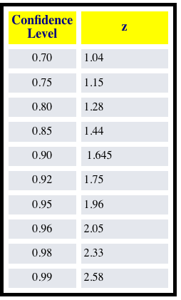
z-score thresholds for different confidence levels:

I've written up this code in my personal project, so I just need to transfer it over to the package:

def z_significance(r1, r2, N, ci='90'):
    """Returns statistical significance between two skill/predictability
    time series.
    Example:
        i_skill = compute_reference(DPLE_dt, FOSI_dt)
        p_skill = compute_persistence(FOSI_dt, 10)
        # N is length of original time series being
        # correlated
        sig = z_significance(i_skill, p_skill, 61)
    """
    def _r_to_z(r):
        return 0.5 * (log(1 + r) - log(1 - r))

    z1, z2 = _r_to_z(r1), _r_to_z(r2)
    difference = np.abs(z1 - z2)
    zo = difference / (2 * sqrt(1 / (N - 3)))
    # Could broadcast better than this, but this works for now.
    confidence = {'80': [1.282]*len(z1),
                  '90': [1.645]*len(z1),
                  '95': [1.96]*len(z1),
                  '99': [2.576]*len(z1)}
    sig = xr.DataArray(zo > confidence[ci], dims='lead time')
    return sig

Can we document what we do in the nc attrs?

when we save skill to skill.nc, we could add the way how we calculated the skill in the nc attributes. To be seen in a terminal with ncdump -h

similar:
https://github.com/NCAR/esmlab/blob/master/esmlab/utils/_variables.py

def get_original_attrs(x):
    attrs = x.attrs.copy()
    encoding = x.encoding
    if "_FillValue" not in encoding:
        encoding["_FillValue"] = None
    return attrs, encoding


def update_attrs(x, original_attrs, original_encoding):
    for att in ["grid_loc", "coordinates"]:
        if att in original_attrs:
            del original_attrs[att]

    x.attrs = original_attrs
    x.encoding = {
        key: val
        for key, val in original_encoding.items()
        if key in ["_FillValue", "dtype"]
    }
return x

I don't have much experience with object-oriented programming, but I should learn. I was thinking it might simplify our code and be powerful to create a "decadal prediction" object.

We could move all our computations to methods within it, similar to how you can run ds.mean().

It could look something like:

dple = load_dple() # this just loads the CESM-DPLE
dp = climpred.decadalPrediction(dple) # could be a different name

dp.compute(hindcast, metric='rmse', comparison='m2r') # an example of what it could look like

Not sure if this would be helpful or not, but just something I've been thinking about

Create some simple commands under climpred.graphics similar to in statsmodels: https://github.com/statsmodels/statsmodels/tree/master/statsmodels/graphics.

This would create skill plots vs. lag, etc. for quick checks.

See https://github.com/bradyrx/climpred/issues/22. Should allow things like PPP and nev to be used with ReferenceEnsemble. Just need to think about what variance we are comparing this to. Uninitialized ensemble, observations, etc?

automatically run tests in a conda test_env

Take advantage of existing: don't reinvent the wheel

• murcss:

  • https://rawgit.com/illing2005/murcss/master/doc/build/html/tutorial.html
  • all calculations based on CDOs
  • built primarily for MPI-ESM Decadal Prediction Project MiKlip
  • can handle Murphy-Eppstein decomposition, bias (really useful for hindcasts)
  • can probabilty be used to create lead year timeseries easily
  • contains:
    • MSESS (Mean Squared Error Skill Score)
    • CRPSS (Continous Ranked Probabillity Skill Score)

• properscoring

  • https://github.com/TheClimateCorporation/properscoring
  • contains:
  • Continuous Ranked Probability Score (CRPS)
  • Brier Score

• https://github.com/PeterRochford/SkillMetrics

  • not applicable to maps?

New metrics should be able to be applied to mapped data (input data dimensions lon, lat, time, ensemble, member) and run fast. Otherwise bootstrapping will not work.

Lets post in this thread metrics we want to see in this package:

It would be nice to have the compute functions in a way that they only check for predictability over the member dimension, so the ensemble dimension is free to be plotted.

Now compute results only time as lead time. Then it would also give ensemble or initialization, so we can get a Lead year timeseries over the ensemble space.

This nicely shows how prediction skill is not constant but very dependent of initialization state.
http://hdl.handle.net/21.11116/0000-0002-0A63-4 Fig. 6.1

Need to adapt computes and remove mean over all ensembles.

Propose: add flag mean_forecast=True as is, as we compute the mean forecast over all init states, and mean_forecast=False for the new part.

To be added to predictionensemble class.
Spatial smoothing, eg. 5x5degree grid
Temporal smoothing, eg. 4yr means
applied to reference and forecast
as in Goddard 2013

See https://github.com/bradyrx/climpred/issues/22. We have a good base of deterministic metrics available, but should eventually add probabilistic metrics that account for initialized ensemble spread.

• pytest (like xskillscore)

What should be tested:

• high-level:
  • do all high-level compute functions work for xr.datasets and xr.dataarrays for all metrics and comparisons (should be done with decorators and tiny synthetic data)
• lower-level:
  • specific functions
    • xr_predictability_horizon (based on the sample output, but that would take long)

Make a vis function for a fan chart

Ref:

import matplotlib.pyplot as plt
import numpy as np

N = 1000
x = np.linspace(0, 10, N)
y = x**2
ones = np.ones(N)

vals = [30, 20, 10] # Values to iterate over and add/subtract from y.

fig, ax = plt.subplots()

for i, val in enumerate(vals):
    alpha = 0.5*(i+1)/len(vals) # Modify the alpha value for each iteration.
    ax.fill_between(x, y+ones*val, y-ones*val, color='red', alpha=alpha)

ax.plot(x, y, color='red') # Plot the original signal

plt.show()

merge comparisons (e2r is basically the same as e2c, m2r is the same as m2c(e), the _x2c functions rely on one input whereas the _x2r functions rely on two inputs)

@aaronspring
Regarding comparisons. The six in the code are very similar:

e2r is methodologically the same as e2c
m2r is methodologically the same as m2c and m2e
m2m is a bit outstanding for PMs

The _x2c functions rely on one input whereas the _x2r functions rely on two inputs.

The ref for PMs can easiliy be split from my original ds input.

I would like to bring those concepts together, because then we can combine the compute function. However, then for PPP and NEV PMs would still need an additional argument compute(dp, ref, control) to give the long control run to the function to assess control.std('time') from a long run.

For m2m I would need a serial approach: First to it m2c or m2r and iterate over all members.

@bradyrx
e2r is methodologically the same as e2c

Is there a difference with the supervector approach though? For my e2r I just take the mean of the DPLE if they provide one with a lot of members. Then compare the DPLE one-to-one with the reference, since we expect/force the reference to be the same length as the DPLE.

With your case, the control is much longer than the DPLE, so you have to take a supervector by repeating the DPLE until it is the length of the control, I think?

Same thoughts for the m2r / m2c comparison.

I do think if we combine these into one function, we should use the x2r terminology, since "reference" can capture a control run, assimilation, hindcast, reconstruction, observations, etc.

I would like to bring those concepts together, because then we can combine the compute function.

I think keeping compute_perfect_model and compute_reference separate is probably good so that the user is very explicit on what type of DP they are using. They might accidentally do a PM instead of an assimilation comparison if it's controlled by some single keyword they (or I) forget to turn on or off.

Regardless, if we combine the comparisons into e2r, m2r, etc. we could have a flag for "PM" vs. "reconstruction" that either takes the supervector approach or not. These flags would automatically be run whether compute_perfect_model or compute_reference is run.

Incorporate a function to compute average predictability time (APT), reference is DelSole

Create a notebook (https://github.com/bradyrx/esmtools/blob/master/notebooks/stats_demo_and_test.ipynb) that demos all of the features in stats.py.

Currently, we have a clean compute_persistence function. We should add a compute_damped_persistence as well.

Write a function to incorporate an f-test significance test for DPP (Pohlmann 2004; Griffies 1977)

I noticed that our nev metric wraps nmse:

def _nmse(ds, control, comparison, running=None, reference_period=None):
    """
    Normalized Ensemble Variance (NEV) metric.
    Reference
    ---------
    - Griffies, S. M., and K. Bryan. “A Predictability Study of Simulated North
      Atlantic Multidecadal Variability.” Climate Dynamics 13, no. 7–8
      (August 1, 1997): 459–87. https://doi.org/10/ch4kc4.
    """
    supervector_dim = 'svd'
    fct, truth = comparison(ds, supervector_dim)
    mse_skill = _mse(fct, truth, dim=supervector_dim)
    var = _get_variance(control, time_length=running,
                        reference_period=reference_period)
    fac = _get_norm_factor(comparison)
    nmse_skill = mse_skill / var / fac
    return nmse_skill

Is this correct? From Ocean Forecasting: Conceptual Basis and Applications, they describe normalzed ensemble variance as the following:

The variance was norrnalized using the variance computed from the control integration.
When the normalized variance reaches unity, the variations between the
individual forecast members are as large as typical variations in the control run,
which defines a predictability limit.

It seems like nev should be something like:

nev = DPLE.var('member') / control.var('time')

And then when nev >= 1, you've reached the predictability limit based on variance.

I like the viz of proplot, but I don't like how it overwrites default settings.

Somehow it changes the defaults of xr.plot() and this slows down the vizualisation of maps drastically. It took me 2min to plot one map. That cannot be. I somehow need to understand this more.

Furthermore, the nice graphics complicates the handling of top-level functions for people who are new to climpred. I think a least-dependency tutorial will be the easiest for us and others.We also additionally provide a fancy proplot version.