hafen / geofacet Goto Github PK
View Code? Open in Web Editor NEWR package for geographical faceting with ggplot2
Home Page: https://hafen.github.io/geofacet/
License: Other
R package for geographical faceting with ggplot2
Home Page: https://hafen.github.io/geofacet/
License: Other


Grid layout for the prefectures of Japan.
Grid data:
"code","code_pref_jis","name","name_abb","name_region","col","row"
"1","01","Hokkaido","HKD","Hokkaido",15,1
"2","02","Aomori","AOM","Tohoku",14,2
"3","03","Iwate","IWT","Tohoku",14,3
"5","05","Akita","AKT","Tohoku",13,3
"4","04","Miyagi","MYG","Tohoku",14,4
"6","06","Yamagata","YGT","Tohoku",13,4
"7","07","Fukushima","FKS","Tohoku",14,5
"8","08","Ibaraki","IBR","Kanto",13,5
"15","15","Niigata","NGT","Chubu",12,5
"9","09","Tochigi","TCG","Kanto",12,6
"10","10","Gunma","GNM","Kanto",14,6
"11","11","Saitama","SIT","Kanto",13,6
"16","16","Toyama","TYM","Chubu",11,6
"17","17","Ishikawa","ISK","Chubu",10,6
"12","12","Chiba","CHB","Kanto",14,7
"13","13","Tokyo","TKY","Kanto",13,7
"18","18","Fukui","FKI","Chubu",10,7
"19","19","Yamanashi","YMN","Chubu",12,7
"20","20","Nagano","NGN","Chubu",11,7
"26","26","Kyoto","KYT","Kinki",9,7
"28","28","Hyogo","HYG","Kinki",8,7
"31","31","Tottori","TTR","Chugoku",7,7
"32","32","Shimane","SMN","Chugoku",6,7
"14","14","Kanagawa","KNG","Kanto",13,8
"21","21","Gifu","GIF","Chubu",10,8
"22","22","Shizuoka","SZO","Chubu",12,8
"23","23","Aichi","AIC","Chubu",11,8
"25","25","Shiga","SIG","Kinki",9,8
"27","27","Osaka","OSK","Kinki",8,8
"33","33","Okayama","OKY","Chugoku",7,8
"34","34","Hiroshima","HRS","Chugoku",6,8
"35","35","Yamaguchi","YGC","Chugoku",5,8
"24","24","Mie","MIE","Chubu",10,9
"29","29","Nara","NAR","Kinki",9,9
"40","40","Fukuoka","FKO","Kyushu / Okinawa",4,9
"41","41","Saga","SAG","Kyushu / Okinawa",3,9
"42","42","Nagasaki","NGS","Kyushu / Okinawa",2,9
"30","30","Wakayama","WKY","Kinki",9,10
"37","37","Kagawa","KGW","Shikoku",7,10
"38","38","Ehime","EHM","Shikoku",6,10
"43","43","Kumamoto","KMM","Kyushu / Okinawa",3,10
"44","44","Oita","OIT","Kyushu / Okinawa",4,10
"36","36","Tokushima","TKS","Shikoku",7,11
"39","39","Kochi","KUC","Shikoku",6,11
"45","45","Miyazaki","MYZ","Kyushu / Okinawa",4,11
"46","46","Kagoshima","KGS","Kyushu / Okinawa",3,11
"47","47","Okinawa","OKN","Kyushu / Okinawa",1,12

[[Note: Please edit the title above and provide a description of the grid here.
Also check the ISO_3166-2 (https://en.wikipedia.org/wiki/ISO_3166-2)
codes if your grid uses countries or states/provinces. Finally, if you can
provide an example of your grid in action with a data set and sample code,
that would be great but is not required. Remove this text before submitting.]]
Grid data:
state,code,row,col
Abia,NG-AB,1,1
Anambra,NG-AN,1,2
Imo,NG-IM,1,5
Enugu,NG-EN,1,4
Ebonyi,NG-EB,1,3
Bayelsa,NG-BY,2,2
Akwa Ibom,NG-AK,2,1
Cross River,NG-CR,2,3
Rivers,NG-RI,2,5
Edo,NG-ED,2,6
Delta,NG-DE,2,4
Ogun,NG-OG,3,3
Ekiti,NG-EK,3,1
Lagos,NG-LA,3,2
Osun,NG-OS,3,5
Oyo,NG-OY,3,6
Ondo,NG-ON,3,4
Nassarawa,NG-NA,4,3
Plateau,NG-PL,4,7
Kwara,NG-KW,4,6
Kogi,NG-KO,4,5
Benue,NG-BE,4,2
Abuja,NG-FC,4,1
Niger,NG-NI,4,4
Bauchi,NG-BA,5,2
Adamawa,NG-AD,5,1
Borno,NG-BO,5,4
Taraba,NG-TA,5,5
Gombe,NG-GO,5,3
Yobe,NG-YO,5,6
Katsina,NG-KT,6,4
Kaduna,NG-KD,6,2
Kano,NG-KN,6,3
Sokoto,NG-SO,6,6
Zamfara,NG-ZA,6,7
Kebbi,NG-KE,6,5
Jigawa,NG-JI,6,1
This is a grid for the German states ("Länder")
Grid data:
row,col,code,name,name_de
1,2,SH,Schleswig-Holstein,Schleswig-Holstein
1,3,HH,Hamburg,Hamburg
1,4,MV,Mecklenburg-Vorpommern,Mecklenburg-Vorpommern
2,2,HB,Bremen,Bremen
2,3,NI,Lower Saxony,Niedersachen
2,4,BE,Berlin,Berlin
2,5,BB,Brandenburg,Brandenburg
3,2,NW,North Rhine-Westphalia,Nordrhein-Westphalen
3,4,ST,Saxony-Anhalt,Sachsen-Anhalt
4,1,SL,Saarland,Saarland
4,2,RP,Rhineland-Palatinate,Rheinland-Pfalz
4,3,HE,Hesse,Hessen
4,4,TH,Thuringia,Thüringen
4,5,SN,Saxony,Sachsen
5,3,BW,Baden-Württemberg,Baden-Württemberg
5,4,BY,Bavaria,Bayern
[[Note: Please edit the title above and provide a description of the grid here.
Also check the ISO_3166-2 (https://en.wikipedia.org/wiki/ISO_3166-2)
codes if your grid uses countries or states/provinces. Finally, if you can
provide an example of your grid in action with a data set and sample code,
that would be great but is not required. Remove this text before submitting.]]
Grid data:
row,col,code,state,sex_eatio,growth_rate
1,11,NG-KD,Kaduna,105.3,3.1
1,10,NG-ON,Ondo,104.9,3.0
2,2,NG-EB,Ebonyi, 91.9,2.8
2,6,NG-ED,Edo,104.0,2.8
2,10,NG-KT,Katsina,105.9,3.0
2,7,NG-KE,Kebbi, 99.8,3.2
2,5,NG-KO,Kogi,106.6,3.0
2,3,NG-NA,Nassarawa,103.0,3.1
2,9,NG-PL,Plateau,100.5,2.9
2,4,NG-SO,Sokoto,102.6,3.0
3,10,NG-BY,Bayelsa,112.7,2.9
3,6,NG-EK,Ekiti,103.5,3.1
3,5,NG-EN,Enugu, 99.5,3.0
3,2,NG-OG,Ogun, 98.2,3.3
3,9,NG-OS,Osun,103.4,3.2
3,7,NG-TA,Taraba,109.0,2.9
3,1,NG-ZA,Zamfara,100.1,3.2
4,1,NG-AN,Anambra,108.3,2.8
4,3,NG-BA,Bauchi,107.8,3.4
4,10,NG-BE,Benue,105.3,3.0
4,6,NG-IM,Imo,106.8,3.2
4,9,NG-KN,Kano,106.7,3.4
4,5,NG-LA,Lagos,107.9,3.2
4,4,NG-NI,Niger,106.0,3.4
5,2,NG-AD,Adamawa,102.8,2.9
5,5,NG-AK,Akwa Ibom,109.0,3.4
5,4,NG-GO,Gombe,109.6,3.2
5,3,NG-OY,Oyo,101.0,3.4
5,7,NG-RI,Rivers,109.5,3.4
6,7,NG-AB,Abia,102.5,2.8
6,8,NG-CR,Cross River,106.9,2.9
6,5,NG-JI,Jigawa,103.9,2.9
6,6,NG-KW,Kwara,106.1,3.0
6,4,NG-YO,Yobe,108.1,3.5
7,2,NG-FC,Abuja,111.4,9.3
7,9,NG-BO,Borno,108.6,3.5
7,1,NG-DE,Delta,102.5,3.2

Grid for Malaysian states and territories
Grid data:
name,code,row,col
Perlis,MY-09,1,1
Pulau Pinang,MY-07,2,1
Kedah,MY-02,2,2
Kelantan,MY-03,2,3
W.P Labuan,MY-15,2,5
Perak,MY-08,3,2
Terengganu,MY-11,3,3
Sabah,MY-12,3,6
Selangor,MY-10,4,2
Pahang,MY-06,4,3
Sarawak,MY-13,4,5
W.P. Kuala Lumpur,MY-14,5,2
W.P.Putrajaya,MY-16,5,3
Negeri Sembilan,MY-05,6,2
Melaka,MY-04,6,3
Johor,MY-01,7,4
Nigeria grid newly created
[[Note: To help streamline the process of adding this grid, please replace this text with an image of a map for the region for reference. Also, please check the ISO_3166-2 (https://en.wikipedia.org/wiki/ISO_3166-2) codes if your grid uses countries or states/provinces. Finally, if you can provide an example of your grid in action with a data set and sample code, that would be great but is not required.]]
Grid data:
"row","col","code","name"
6,7,"NG-AB","Abia"
7,2,"NG-FC","Abuja"
5,2,"NG-AD","Adamawa"
5,5,"NG-AK","Akwa Ibom"
4,1,"NG-AN","Anambra"
4,3,"NG-BA","Bauchi"
3,10,"NG-BY","Bayelsa"
4,10,"NG-BE","Benue"
7,9,"NG-BO","Borno"
6,8,"NG-CR","Cross River"
7,1,"NG-DE","Delta"
2,2,"NG-EB","Ebonyi"
2,6,"NG-ED","Edo"
3,6,"NG-EK","Ekiti"
3,5,"NG-EN","Enugu"
5,4,"NG-GO","Gombe"
4,6,"NG-IM","Imo"
6,5,"NG-JI","Jigawa"
1,11,"NG-KD","Kaduna"
4,9,"NG-KN","Kano"
2,10,"NG-KT","Katsina"
2,7,"NG-KE","Kebbi"
2,5,"NG-KO","Kogi"
6,6,"NG-KW","Kwara"
4,5,"NG-LA","Lagos"
2,3,"NG-NA","Nassarawa"
4,4,"NG-NI","Niger"
3,2,"NG-OG","Ogun"
1,10,"NG-ON","Ondo"
3,9,"NG-OS","Osun"
5,3,"NG-OY","Oyo"
2,9,"NG-PL","Plateau"
5,7,"NG-RI","Rivers"
2,4,"NG-SO","Sokoto"
3,7,"NG-TA","Taraba"
6,4,"NG-YO","Yobe"
3,1,"NG-ZA","Zamfara"
[[Note: Please edit the title above and provide a description of the grid here.
Also check the ISO_3166-2 (https://en.wikipedia.org/wiki/ISO_3166-2)
codes if your grid uses countries or states/provinces. Finally, if you can
provide an example of your grid in action with a data set and sample code,
that would be great but is not required. Remove this text before submitting.]]
Grid data:
    state  code sex_ratio growth_rate,row,col
1         Abia NG-AB     102.5         2.8,1,1
2        Abuja NG-FC     111.4         9.3,1,2
3      Adamawa NG-AD     102.8         2.9,1,3
4    Akwa Ibom NG-AK     109.0         3.4,1,4
5      Anambra NG-AN     108.3         2.8,1,5
6       Bauchi NG-BA     107.8         3.4,1,6
7      Bayelsa NG-BY     112.7         2.9,1,7
8        Benue NG-BE     105.3         3.0,1,8
9        Borno NG-BO     108.6         3.5,2,1
10 Cross River NG-CR     106.9         2.9,2,2
11       Delta NG-DE     102.5         3.2,2,3
12      Ebonyi NG-EB      91.9         2.8,2,4
13         Edo NG-ED     104.0         2.8,2,5
14       Ekiti NG-EK     103.5         3.1,2,6
15       Enugu NG-EN      99.5         3.0,2,7
16       Gombe NG-GO     109.6         3.2,2,8
17         Imo NG-IM     106.8         3.2,3,1
18      Jigawa NG-JI     103.9         2.9,3,2
19      Kaduna NG-KD     105.3         3.1,3,3
20        Kano NG-KN     106.7         3.4,3,4
21     Katsina NG-KT     105.9         3.0,3,5
22       Kebbi NG-KE      99.8         3.2,3,6
23        Kogi NG-KO     106.6         3.0,3,7
24       Kwara NG-KW     106.1         3.0,3,8
25       Lagos NG-LA     107.9         3.2,4,1
26   Nassarawa NG-NA     103.0         3.1,4,2
27       Niger NG-NI     106.0         3.4,4,3
28        Ogun NG-OG      98.2         3.3,4,4
29        Ondo NG-ON     104.9         3.0,4,5
30        Osun NG-OS     103.4         3.2,4,6
31         Oyo NG-OY     101.0         3.4,4,7
32     Plateau NG-PL     100.5         2.9,4,8
33      Rivers NG-RI     109.5         3.4,5,1
34      Sokoto NG-SO     102.6         3.0,5,2
35      Taraba NG-TA     109.0         2.9,5,3
36        Yobe NG-YO     108.1         3.5,5,4
37     Zamfara NG-ZA     100.1         3.2,5,5
Grid for the 23 provinces of Argentina. It includes the Malvinas/Falkland Islands and the Antarctic Territories (these are disputed, but I think they should still be included since many researchers might use data from that location).
Grid data:
"code","code_short","name_es","col","row"
"AR-B","B","Buenos Aires",3,5
"AR-C","C","Ciudad Autónoma de Buenos Aires",4,5
"AR-K","K","Catamarca",1,3
"AR-H","H","Chaco",3,3
"AR-U","U","Chubut",1,8
"AR-X","X","Córdoba",2,4
"AR-W","W","Corrientes",4,3
"AR-E","E","Entre Ríos",4,4
"AR-P","P","Formosa",3,2
"AR-Y","Y","Jujuy",1,1
"AR-L","L","La Pampa",2,6
"AR-F","F","La Rioja",1,4
"AR-M","M","Mendoza",1,6
"AR-N","N","Misiones",5,2
"AR-Q","Q","Neuquén",1,7
"AR-R","R","Río Negro",2,7
"AR-A","A","Salta",1,2
"AR-J","J","San Juan",1,5
"AR-D","D","San Luis",2,5
"AR-Z","Z","Santa Cruz",1,9
"AR-S","S","Santa Fe",3,4
"AR-G","G","Santiago del Estero",2,3
"AR-V","V","Tierra del Fuego",1,10
"AR-T","T","Tucumán",2,2
"FK","FK","Islas Malvinas",4,9
"AQ","AQ","Antártida Argentina",2,12
Codes:
https://www.iso.org/obp/ui/#iso:code:3166:AR
Map:
(from the National Geographic Institute)
library(data.table)
library(ggplot2)
library(geofacet)

# From https://www.iso.org/obp/ui/#iso:code:3166:AR
argentina_grid <- fread("~/Dropbox/R/argentina_grid.csv")
arg_labels <- setNames(argentina_grid$name, argentina_grid$code)

arg.data <- data.table(prov = rep(argentina_grid$code, 12))
arg.data[, c("pp", "month") := .(rnorm(12), 1:12), by = prov]

ggplot(arg.data, aes(month, pp)) +
    geom_point() +
    # facet_wrap(~prov)
    coord_equal() +
facet_geo(~prov, grid = argentina_grid) Grid data for Nepal's 75 districts:
row,col,code,name
1,4, NP01, Humla
1,5, NP02, Mugu
1,6, NP03, Dolpa
1,7, NP04, Mustang
1,8, NP05, Manang
2,9, NP06, Gorkha
2,1, NP07, Dharchula
2,2, NP08, Bajhang
2,3, NP09, Bajura
2,4, NP10, Kalikot
2,5, NP11, Jumla
2,6, NP12, Rukum
2,7, NP13, Myagdi
2,8, NP14, Kaski
2,10, NP15, Dhading
2,11, NP16, Rasuwa
2,12, NP17, Sindhupalchowk
2,13, NP18, Dolakha
2,14, NP19, Solukhumbu
2,15, NP20, Sankhuwasabha
2,16, NP21, Taplejung
3,9, NP22, Lamjung
3,1, NP23, Baitadi
3,2, NP24, Doti
3,3, NP25, Achham
3,4, NP26, Dailekh
3,5, NP27, Jajarkot
3,6, NP28, Rolpa
3,7, NP29, Baglung
3,8, NP30, Parbat
3,10, NP31, Nuwakot
3,11, NP32, Kavrepalanchok
3,12, NP33, Kathmandu
3,13, NP34, Okhaldhunga
3,14, NP35, Khotang
3,15, NP36, Bhojpur
3,16, NP37, Dhankuta
3,17, NP38, Tehrathum
4,9, NP39, Tanahun
4,1, NP40, Kanchanpur
4,2, NP41, Dadeldhura
4,3, NP42, Kailali
4,4, NP43, Surkhet
4,5, NP44, Salyan
4,6, NP45, Pyuthan
4,7, NP46, Gulmi
4,8, NP47, Syangja
4,10, NP48, Chitwan
4,11, NP49, Patan
4,12, NP50, Bhaktapur
4,13, NP51, Ramechhap
4,14, NP52, Udayapur
4,15, NP53, Sunsari
4,16, NP54, Panchthar
4,17, NP55, Ilam
5,9, NP56, Nawalparasi
5,4, NP57, Bardiya
5,5, NP58, Banke
5,6, NP59, Dang
5,7, NP60, Argakhanchi
5,8, NP61, Palpa
5,10, NP62, Parsa
5,11, NP63, Makwanpur
5,12, NP64, Sindhuli
5,13, NP65, Dhanussa
5,14, NP66, Siraha
5,15, NP67, Saptari
5,16, NP68, Morang
5,17, NP69, Jhapa
6,7, NP70,  Kapilvastu
6,8, NP71, Rupandehi
6,10, NP72, Bara
6,11, NP73, Rahuttahat
6,12, NP74, Sarlahi
6,13, NP75, Mahottari
South African Provinces
"code","row","col","name"
"WC",4,1,"Western Cape"
"EC",4,2,"Eastern Cape"
"NC",3,1,"Northern Cape"
"GP",2,2,"Gauteng"
"KZN",3,3,"KwaZulu-Natal"
"MP",2,3,"Mpumalanga"
"LP",1,3,"Limpopo"
"NW",2,1,"North West"
"FS",3,2,"Free State"

Code to produce the above example
With thanks to @jonocarroll whose prior effort paved the way and made this easy.
As seen in an article by the Washington Post.
Example code:
library(tidyverse)
library(geofacet)
library(ggthemes)
options(scipen = 99)

us_state_grid4 <- data.frame(
  row = c(1, 1, 2, 2, 2, 3, 3, 3, 3, 3, 3, 3, 3, 3, 4, 4, 4, 4, 4, 4, 4, 4, 4, 4, 4, 5, 5, 5, 5, 5, 5, 5, 5, 5, 5, 6, 6, 6, 6, 6, 6, 6, 6, 7, 7, 7, 7, 7, 8, 8, 8),
  col = c(11, 1, 11, 10, 6, 2, 6, 10, 7, 5, 3, 9, 4, 1, 10, 6, 5, 2, 9, 7, 1, 8, 11, 4, 3, 1, 3, 10, 6, 9, 5, 4, 2, 8, 7, 2, 5, 4, 3, 7, 8, 6, 9, 7, 8, 5, 6, 4, 9, 1, 4),
  code = c("ME", "AK", "NH", "VT", "WI", "ID", "IL", "MA", "MI", "MN", "MT", "NY", "ND", "WA", "CT", "IN", "IA", "NV", "NJ", "OH", "OR", "PA", "RI", "SD", "WY", "CA", "CO", "DE", "KY", "MD", "MO", "NE", "UT", "VA", "WV", "AZ", "AR", "KS", "NM", "NC", "SC", "TN", "DC", "AL", "GA", "LA", "MS", "OK", "FL", "HI", "TX"),
  name = c("Maine", "Alaska", "New Hampshire", "Vermont", "Wisconsin", "Idaho", "Illinois", "Massachusetts", "Michigan", "Minnesota", "Montana", "New York", "North Dakota", "Washington", "Connecticut", "Indiana", "Iowa", "Nevada", "New Jersey", "Ohio", "Oregon", "Pennsylvania", "Rhode Island", "South Dakota", "Wyoming", "California", "Colorado", "Delaware", "Kentucky", "Maryland", "Missouri", "Nebraska", "Utah", "Virginia", "West Virginia", "Arizona", "Arkansas", "Kansas", "New Mexico", "North Carolina", "South Carolina", "Tennessee", "District of Columbia", "Alabama", "Georgia", "Louisiana", "Mississippi", "Oklahoma", "Florida", "Hawaii", "Texas"),
  stringsAsFactors = FALSE
)

state_rates <- read.csv("https://gist.githubusercontent.com/kanishkamisra/9f7677a7ec05984d060260066eb02d53/raw/64da90856d3ab4f623bbbfdcf94e81b517baefd1/state_mortality")
usa_rates <- read.csv("https://gist.githubusercontent.com/kanishkamisra/a2f49ec4c037751dad94fe8a58dff691/raw/810edc2bc06e4a9a24ec80d5ab729935cee7a9d1/usa_rate.csv")

usa_joining <- usa_rates %>%
  transmute(
    year_id,
    usa_rate = mx,
    usa_avg = mx
  )

usa_vs_state <- state_rates %>%
  transmute(
    location_name,
    year_id,
    state_rate = mx,
    state_avg = mx
  ) %>%
  inner_join(
    usa_joining,
    by = c("year_id")
  ) %>%
  # Little trick to get the geom_ribbon fill color to be the color of the
  # higher rate (USA avg or state avg) in any given year.
  # That is why I have two columns for the same rate value.
  # One is used to gather and plot (ymin in the ribbon)
  # the other is to specify the ribbon ymax value.
  # Might not be the most elegant way to do it in a larger dataset.
  gather(state_rate, usa_rate, key = "metric", value = "value") %>%
  separate(metric,into = c("metric", "extra")) %>%
  select(-extra) %>%
  mutate(
    ribbon_color = case_when(
      state_avg > usa_avg ~ "#f8766d",
      usa_avg > state_avg ~ "#00bfc4"
    ),
    ribbon_value = case_when(
      state_avg > usa_avg ~ state_avg,
      usa_avg > state_avg ~ usa_avg
    )
  )

usa_vs_state %>%
  ggplot(aes(year_id, value, color = metric)) +
  geom_line(size = 1) +
  geom_ribbon(aes(ymin = value, ymax = ribbon_value, linetype = NA, fill = ribbon_color), alpha = 0.2, show.legend = F) +
  facet_geo(~location_name, grid = us_state_grid4) +
  scale_fill_identity() +
  theme_fivethirtyeight() +
  theme(legend.position = "top",
        legend.margin = margin(b = -1, unit = "cm")) +
  labs(
    x = "Year",
    y = "Mortality Rate",
    title = "Mortality Rates in each state vs U.S. average, 1980-2014",
    subtitle = "Deaths per 100,000 people",
    color = "Rate",
    caption = "By Kanishka Misra    Source: IHME"
  )

# ggsave("usa_vs_state1.png", height = 10, width = 17)
Example Resulting Plot:

Grid data:
row,col,code,name
1,11,ME,Maine
1,1,AK,Alaska
2,11,NH,New Hampshire
2,10,VT,Vermont
2,6,WI,Wisconsin
3,2,ID,Idaho
3,6,IL,Illinois
3,10,MA,Massachusetts
3,7,MI,Michigan
3,5,MN,Minnesota
3,3,MT,Montana
3,9,NY,New York
3,4,ND,North Dakota
3,1,WA,Washington
4,10,CT,Connecticut
4,6,IN,Indiana
4,5,IA,Iowa
4,2,NV,Nevada
4,9,NJ,New Jersey
4,7,OH,Ohio
4,1,OR,Oregon
4,8,PA,Pennsylvania
4,11,RI,Rhode Island
4,4,SD,South Dakota
4,3,WY,Wyoming
5,1,CA,California
5,3,CO,Colorado
5,10,DE,Delaware
5,6,KY,Kentucky
5,9,MD,Maryland
5,5,MO,Missouri
5,4,NE,Nebraska
5,2,UT,Utah
5,8,VA,Virginia
5,7,WV,West Virginia
6,2,AZ,Arizona
6,5,AR,Arkansas
6,4,KS,Kansas
6,3,NM,New Mexico
6,7,NC,North Carolina
6,8,SC,South Carolina
6,6,TN,Tennessee
6,9,DC,District of Columbia
7,7,AL,Alabama
7,8,GA,Georgia
7,5,LA,Louisiana
7,6,MS,Mississippi
7,4,OK,Oklahoma
8,9,FL,Florida
8,1,HI,Hawaii
8,4,TX,Texas
Grid for Nigeria's 37 Federal Staes
Grid data:
row,col,code,name
1,4,NG.KT,Katsina
1,5, NG.KN, Kano
1,2,NG.SO,Sokoto
1,3, NG.ZA, Zamfara
1,6, NG.JI, Jigawa
1,7, NG.YO, Yobe
2,2, NG.KE, Kebbi
2,3, NG.NI, Niger
2,4, NG.KD, Kaduna
2,7, NG.BO, Borno
2,6, NG.GO, Gombe
2,5, NG.BA, Bauchi
3,1, NG.OY, Oyo
3,2, NG.KW, Kwara
3,3,NG.FC, Abuja FCT
3,4, NG.NA, Nassarawa
3,6, NG.AD, Adamawa
3,5, NG.PL, Plateau
4,3, NG.EK, Ekiti
4,1, NG.OG, Ogun
4,2, NG.OS, Osun
4,4, NG.KO, Kogi
4,6, NG.TA, Taraba
4,5, NG.BE, Benue
5,3,NG.ED, Edo
5,1, NG.LA, Lagos
5,2, NG.ON, Ondo
5,6,NG.EB, Ebonyi
5,4, NG.AN, Anambra
5,5, NG.EN, Enugu
6,2, NG.DE, Delta
6,3, NG.IM, Imo
6,4,NG.AB, Abia
6,5, NG.CR, Cross River
7,3, NG.BY, Bayelsa
7,4, NG.RI, Rivers
7,5, NG.AK, Akwa Ibom
Grid for South East Asian countries
Grid data:
name,code,row,col
Laos,LA,1,2
Myanmar,MM,1,1
Vietnam,VN,1,3
Thailand,TH,2,1
Cambodia,KH,2,2
Philippines,PH,2,4
Brunei,BN,3,3
Malaysia,MY,3,1
Singapore,SG,4,2
East Timor,TL,5,4
Indonesia,ID,5,3
Creating a grid is not an exact science and probably most of the time there will be the need for manual tweaking. How about integrating a tool for creating a grid?
I've tried something here: https://ecamp.shinyapps.io/grid_create/
It's barely usable, the leftmost table doesn't update and there's not way to download the new grid or to add or remove codes. But it's only a start. What do you think?
Grid data:
code,county,row,col
18011,Boone,1,2
18057,Hamilton,1,3
18095,Madison,1,4
18133,Putnam,2,1
18059,Hancock,2,4
18097,Marion,2,3
18063,Hendricks,2,2
18109,Morgan,3,2
18081,Johnson,3,3
18145,Shelby,3,4
18013,Brown,4,3
Land and overseas regions of France
Insee codes.
Grid data:
"code_region","name_region","row","col"
"01","Guadeloupe",1,7
"32","Hauts-de-France",1,3
"11","Île-de-France",2,3
"02","Martinique",2,7
"44","Grand Est",2,5
"28","Normandie",2,2
"27","Bourgogne-Franche-Comté",2,4
"53","Bretagne",2,1
"24","Centre-Val de Loire",3,3
"52","Pays de la Loire",3,2
"03","Guyane",3,7
"84","Auvergne-Rhône-Alpes",3,4
"75","Nouvelle-Aquitaine",4,2
"76","Occitanie",4,3
"93","Provence-Alpes-Côte d'Azur",4,4
"04","Réunion",4,7
"06","Mayotte",5,7
"94","Corse",5,5
An example with GDP per capita :

Australian States and Territories; an alternative grid with less whitespace.
"code","row","col","name"
"WA",2,1,"Western Australia"
"NT",1,2,"Northern Territory"
"SA",2,2,"South Australia"
"QLD",1,3,"Queensland"
"NSW",2,3,"New South Wales"
"ACT",3,4,"Australian Capital Territory"
"VIC",3,3,"Victoria"
"TAS",4,3,"Tasmania"

geofacet grid for Bangladesh 64 Upazilas
Grid data:
row,col,code,name
1,3, BG01, Panchagar
2,2, BG02, Takurgaong
2,3, BG03, Nilphamar
2,4, BG04, Lamonirhat
3,3, BG05, Dinajpur
3,4, BG06, Rangpur
3,5, BG07, Kurigram
4,3, BG08, Jaipurat
4,4, BG09, Gaibandha
5,2, BG10, Naogaon
5,3, BG11, Bogra
5,4, BG12, Jamalpur
5,5,BG13, Sherpar
5,6,BG14, Mymensingh
5,7,BG15, Netrokona
5,8, BG16, Suramganj
5,9,BG17, Sylhet
6,1,BG18, Chapai
6,2,BG19,Rajshani
6,3,BG20,Nator
6,4,BG21,Sirajganj
6,5,BG22, Tangail
6,6,BG23, Gazipur
6,7,BG24, Kishoreganj
6,8,BG25, Habiganj
6,9,BG26, Moulvibazar
7,2,BG27, Kushtia
7,3,BG28, Pabna
7,4,BG29, Dhaka
7,5,BG30, Nardiaganj
7,6,BG31, Narsingdi
7,7,BG32, Brahmanbaria
8,1,BG33, Meherpur
8,2,BG34, Jhenaidah
8,3,BG35, Magura
8,4,BG36, Rajbari
8,5,BG37, Manikganj
8,6,BG38, Munshiganj
8,7,BG39, Comilla
9,9,BG40, Khagrachhari
9,10,BG41, Rangramati
9,1,BG42, Chuadanga
9,2,BG43, Jessore
9,3,BG44, Gopalganj
9,4,BG45, Faridpur
9,5,BG46, Madanipur
9,6,BG47, Shariyapur
9,7,BG48, Chandpur
9,8,BG49, Feni
10,9,BG50, Chittagong
10,10,BG51, Badanbari
10,2,BG52, Narail
10,3,BG53, Pirojpur
10,4,BG54, Barisal
10,5,BG55, Jhalkati
10,6,BG56, Laksimipur
10,7,BG57, Noakhali
11,2,BG58, Satkhira
11,3,BG59, Khulna
11,4,BG60, Bagerhat
11,5,BG61, Borguna
11,6,BG62, Patuakhali
11,7,BG63, Bhola
11,9,BG64, Cox's Bazar
    row = c(1, 2, 2, 2, 3, 3, 3, 4, 4, 5, 5, 5, 5, 5, 5, 5, 5, 6, 6, 6, 6, 6, 6, 6, 6, 6, 7, 7, 7, 7, 7, 7, 8, 8, 8, 8, 8, 8, 8, 9, 9, 9, 9, 9, 9, 9, 9, 9, 9, 10, 10, 10, 10, 10, 10, 10, 10, 11, 11, 11, 11, 11, 11, 11),
    col = c(3, 2, 3, 4, 3, 4, 5, 3, 4, 2, 3, 4, 5, 6, 7, 8, 9, 1, 2, 3, 4, 5, 6, 7, 8, 9, 2, 3, 4, 5, 6, 7, 1, 2, 3, 4, 5, 6, 7, 9, 10, 1, 2, 3, 4, 5, 6, 7, 8, 9, 10, 2, 3, 4, 5, 6, 7, 2, 3, 4, 5, 6, 7, 9),
    code = c("BG01","BG02","BG03","BG04","BG05","BG06","BG07","BG08","BG09","BG10","BG11","BG12","BG13","BG14","BG15","BG16","BG17","BG18","BG19","BG20","BG21","BG22","BG23","BG24","BG25","BG26","BG27","BG28","BG29","BG30","BG31","BG32","BG33","BG34","BG35","BG36","BG37","BG38","BG39","BG40","BG41","BG42","BG43","BG44","BG45","BG46","BG47","BG48","BG49","BG50","BG51","BG52","BG53","BG54","BG55","BG56","BG57","BG58","BG59","BG60","BG61","BG62","BG63", "BG64"),
    name = c("Panchagar","Takurgaong","Nilphamar","Lamonirhat","Dinajpur","Rangpur","Kurigram","Jaipurat","Gaibandha","Naogaon","Bogra","Jamalpur","Sherpar","Mymensingh","Netrokona","Suramganj","Sylhet","Chapai","Rajshani","Nator","Sirajganj","Tangail","Gazipur","Kishoreganj","Habiganj","Moulvibazar","Kushtia","Pabna","Dhaka","Nardiaganj","Narsingdi","Brahmanbaria","Meherpur","Jhenaidah","Magura","Rajbari","Manikganj","Munshiganj","Comilla","Khagrachhari","Rangramati","Chuadanga","Jessore","Gopalganj","Faridpur","Madanipur","Shariyapur","Chandpur","Feni","Chittagong","Badanbari","Narail","Pirojpur","Barisal","Jhalkati","Laksimipur","Noakhali","Satkhira","Khulna","Bagerhat","Borguna","Patuakhali","Bhola","Cox's Bazar"),
    stringsAsFactors = FALSE
  )

geofacet::grid_preview(mygrid)
library(tidyverse)
library(geofacet)
library(ggthemes)
options(scipen = 99)
p <- ggplot(dt3 , aes(type, value, fill=type))+
  geom_col(position = position_dodge())+
  scale_fill_manual(values = c("#7fc97f", "#beaed4","#fdc086","#ffff99"))+
  theme_bw()+
  theme(axis.text.x=element_text(angle = 90, hjust = 0))+
  facet_geo(~name, grid = mygrid) +
  labs(
    x = "Education",
    y = "Percent",
    title = "Bangladesh Education",
    color = "type",
    caption = "By Aledemogr    Source: World Bank"
  )
ggsave("bgd1.png", p,height = 17, width = 14)

dt3<-structure(list(ordinal = c(58L, 58L, 58L, 58L, 58L, 58L, 58L,
34L, 56L, 57L, 34L, 56L, 57L, 34L, 56L, 57L, 34L, 56L, 57L, 34L,
56L, 57L, 34L, 56L, 57L, 34L, 56L, 57L, 53L, 55L, 59L, 53L, 55L,
59L, 53L, 55L, 59L, 53L, 55L, 59L, 53L, 55L, 59L, 53L, 55L, 59L,
53L, 55L, 59L, 47L, 54L, 47L, 54L, 47L, 54L, 47L, 54L, 47L, 54L,
47L, 54L, 47L, 54L, 22L, 27L, 30L, 33L, 45L, 48L, 63L, 64L, 22L,
27L, 30L, 33L, 45L, 48L, 63L, 64L, 22L, 27L, 30L, 33L, 45L, 48L,
63L, 64L, 22L, 27L, 30L, 33L, 45L, 48L, 63L, 64L, 22L, 27L, 30L,
33L, 45L, 48L, 63L, 64L, 22L, 27L, 30L, 33L, 45L, 48L, 63L, 64L,
22L, 27L, 30L, 33L, 45L, 48L, 63L, 64L, 20L, 23L, 46L, 49L, 51L,
52L, 60L, 61L, 62L, 20L, 23L, 46L, 49L, 51L, 52L, 60L, 61L, 62L,
20L, 23L, 46L, 49L, 51L, 52L, 60L, 61L, 62L, 20L, 23L, 46L, 49L,
51L, 52L, 60L, 61L, 62L, 20L, 23L, 46L, 49L, 51L, 52L, 60L, 61L,
62L, 20L, 23L, 46L, 49L, 51L, 52L, 60L, 61L, 62L, 20L, 23L, 46L,
49L, 51L, 52L, 60L, 61L, 62L, 8L, 18L, 28L, 29L, 40L, 50L, 8L,
18L, 28L, 29L, 40L, 50L, 8L, 18L, 28L, 29L, 40L, 50L, 8L, 18L,
28L, 29L, 40L, 50L, 8L, 18L, 28L, 29L, 40L, 50L, 8L, 18L, 28L,
29L, 40L, 50L, 8L, 18L, 28L, 29L, 40L, 50L, 11L, 25L, 26L, 31L,
38L, 41L, 42L, 11L, 25L, 26L, 31L, 38L, 41L, 42L, 11L, 25L, 26L,
31L, 38L, 41L, 42L, 11L, 25L, 26L, 31L, 38L, 41L, 42L, 11L, 25L,
26L, 31L, 38L, 41L, 42L, 11L, 25L, 26L, 31L, 38L, 41L, 42L, 11L,
25L, 26L, 31L, 38L, 41L, 42L, 9L, 13L, 14L, 17L, 19L, 21L, 24L,
32L, 36L, 37L, 9L, 13L, 14L, 17L, 19L, 21L, 24L, 32L, 36L, 37L,
9L, 13L, 14L, 17L, 19L, 21L, 24L, 32L, 36L, 37L, 9L, 13L, 14L,
17L, 19L, 21L, 24L, 32L, 36L, 37L, 9L, 13L, 14L, 17L, 19L, 21L,
24L, 32L, 36L, 37L, 9L, 13L, 14L, 17L, 19L, 21L, 24L, 32L, 36L,
37L, 9L, 13L, 14L, 17L, 19L, 21L, 24L, 32L, 36L, 37L, 2L, 4L,
6L, 7L, 10L, 15L, 16L, 43L, 2L, 4L, 6L, 7L, 10L, 15L, 16L, 43L,
2L, 4L, 6L, 7L, 10L, 15L, 16L, 43L, 2L, 4L, 6L, 7L, 10L, 15L,
16L, 43L, 2L, 4L, 6L, 7L, 10L, 15L, 16L, 43L, 2L, 4L, 6L, 7L,
10L, 15L, 16L, 43L, 2L, 4L, 6L, 7L, 10L, 15L, 16L, 43L, 1L, 3L,
5L, 12L, 35L, 39L, 44L, 1L, 3L, 5L, 12L, 35L, 39L, 44L, 1L, 3L,
5L, 12L, 35L, 39L, 44L, 1L, 3L, 5L, 12L, 35L, 39L, 44L, 1L, 3L,
5L, 12L, 35L, 39L, 44L, 1L, 3L, 5L, 12L, 35L, 39L, 44L, 1L, 3L,
5L, 12L, 35L, 39L, 44L), Division.Name = structure(c(6L, 6L,
6L, 6L, 6L, 6L, 6L, 3L, 6L, 6L, 3L, 6L, 6L, 3L, 6L, 6L, 3L, 6L,
6L, 3L, 6L, 6L, 3L, 6L, 6L, 3L, 6L, 6L, 6L, 6L, 6L, 6L, 6L, 6L,
6L, 6L, 6L, 6L, 6L, 6L, 6L, 6L, 6L, 6L, 6L, 6L, 6L, 6L, 6L, 5L,
6L, 5L, 6L, 5L, 6L, 5L, 6L, 5L, 6L, 5L, 6L, 5L, 6L, 3L, 3L, 3L,
3L, 5L, 5L, 7L, 7L, 3L, 3L, 3L, 3L, 5L, 5L, 7L, 7L, 3L, 3L, 3L,
3L, 5L, 5L, 7L, 7L, 3L, 3L, 3L, 3L, 5L, 5L, 7L, 7L, 3L, 3L, 3L,
3L, 5L, 5L, 7L, 7L, 3L, 3L, 3L, 3L, 5L, 5L, 7L, 7L, 3L, 3L, 3L,
3L, 5L, 5L, 7L, 7L, 3L, 3L, 5L, 5L, 5L, 5L, 6L, 7L, 7L, 3L, 3L,
5L, 5L, 5L, 5L, 6L, 7L, 7L, 3L, 3L, 5L, 5L, 5L, 5L, 6L, 7L, 7L,
3L, 3L, 5L, 5L, 5L, 5L, 6L, 7L, 7L, 3L, 3L, 5L, 5L, 5L, 5L, 6L,
7L, 7L, 3L, 3L, 5L, 5L, 5L, 5L, 6L, 7L, 7L, 3L, 3L, 5L, 5L, 5L,
5L, 6L, 7L, 7L, 2L, 3L, 3L, 3L, 4L, 5L, 2L, 3L, 3L, 3L, 4L, 5L,
2L, 3L, 3L, 3L, 4L, 5L, 2L, 3L, 3L, 3L, 4L, 5L, 2L, 3L, 3L, 3L,
4L, 5L, 2L, 3L, 3L, 3L, 4L, 5L, 2L, 3L, 3L, 3L, 4L, 5L, 2L, 3L,
3L, 3L, 4L, 4L, 4L, 2L, 3L, 3L, 3L, 4L, 4L, 4L, 2L, 3L, 3L, 3L,
4L, 4L, 4L, 2L, 3L, 3L, 3L, 4L, 4L, 4L, 2L, 3L, 3L, 3L, 4L, 4L,
4L, 2L, 3L, 3L, 3L, 4L, 4L, 4L, 2L, 3L, 3L, 3L, 4L, 4L, 4L, 2L,
2L, 2L, 2L, 3L, 3L, 3L, 3L, 4L, 4L, 2L, 2L, 2L, 2L, 3L, 3L, 3L,
3L, 4L, 4L, 2L, 2L, 2L, 2L, 3L, 3L, 3L, 3L, 4L, 4L, 2L, 2L, 2L,
2L, 3L, 3L, 3L, 3L, 4L, 4L, 2L, 2L, 2L, 2L, 3L, 3L, 3L, 3L, 4L,
4L, 2L, 2L, 2L, 2L, 3L, 3L, 3L, 3L, 4L, 4L, 2L, 2L, 2L, 2L, 3L,
3L, 3L, 3L, 4L, 4L, 1L, 1L, 1L, 2L, 2L, 2L, 2L, 4L, 1L, 1L, 1L,
2L, 2L, 2L, 2L, 4L, 1L, 1L, 1L, 2L, 2L, 2L, 2L, 4L, 1L, 1L, 1L,
2L, 2L, 2L, 2L, 4L, 1L, 1L, 1L, 2L, 2L, 2L, 2L, 4L, 1L, 1L, 1L,
2L, 2L, 2L, 2L, 4L, 1L, 1L, 1L, 2L, 2L, 2L, 2L, 4L, 1L, 1L, 1L,
2L, 4L, 4L, 4L, 1L, 1L, 1L, 2L, 4L, 4L, 4L, 1L, 1L, 1L, 2L, 4L,
4L, 4L, 1L, 1L, 1L, 2L, 4L, 4L, 4L, 1L, 1L, 1L, 2L, 4L, 4L, 4L,
1L, 1L, 1L, 2L, 4L, 4L, 4L, 1L, 1L, 1L, 2L, 4L, 4L, 4L), .Label = c("BARISAL",
"CHITTAGONG", "DHAKA", "KHULNA", "RAJSHAHI", "RANGPUR", "SYLHET"
), class = "factor"), Zila.Name = structure(c(50L, 50L, 50L,
50L, 50L, 50L, 50L, 63L, 33L, 47L, 63L, 33L, 47L, 63L, 33L, 47L,
63L, 33L, 47L, 63L, 33L, 47L, 63L, 33L, 47L, 63L, 33L, 47L, 15L,
30L, 56L, 15L, 30L, 56L, 15L, 30L, 56L, 15L, 30L, 56L, 15L, 30L,
56L, 15L, 30L, 56L, 15L, 30L, 56L, 26L, 18L, 26L, 18L, 26L, 18L,
26L, 18L, 26L, 18L, 26L, 18L, 26L, 18L, 22L, 40L, 46L, 59L, 6L,
41L, 61L, 62L, 22L, 40L, 46L, 59L, 6L, 41L, 61L, 62L, 22L, 40L,
46L, 59L, 6L, 41L, 61L, 62L, 22L, 40L, 46L, 59L, 6L, 41L, 61L,
62L, 22L, 40L, 46L, 59L, 6L, 41L, 61L, 62L, 22L, 40L, 46L, 59L,
6L, 41L, 61L, 62L, 22L, 40L, 46L, 59L, 6L, 41L, 61L, 62L, 19L,
29L, 9L, 45L, 54L, 60L, 64L, 21L, 37L, 19L, 29L, 9L, 45L, 54L,
60L, 64L, 21L, 37L, 19L, 29L, 9L, 45L, 54L, 60L, 64L, 21L, 37L,
19L, 29L, 9L, 45L, 54L, 60L, 64L, 21L, 37L, 19L, 29L, 9L, 45L,
54L, 60L, 64L, 21L, 37L, 19L, 29L, 9L, 45L, 54L, 60L, 64L, 21L,
37L, 19L, 29L, 9L, 45L, 54L, 60L, 64L, 21L, 37L, 7L, 14L, 43L,
44L, 31L, 49L, 7L, 14L, 43L, 44L, 31L, 49L, 7L, 14L, 43L, 44L,
31L, 49L, 7L, 14L, 43L, 44L, 31L, 49L, 7L, 14L, 43L, 44L, 31L,
49L, 7L, 14L, 43L, 44L, 31L, 49L, 7L, 14L, 43L, 44L, 31L, 49L,
12L, 36L, 39L, 53L, 25L, 35L, 38L, 12L, 36L, 39L, 53L, 25L, 35L,
38L, 12L, 36L, 39L, 53L, 25L, 35L, 38L, 12L, 36L, 39L, 53L, 25L,
35L, 38L, 12L, 36L, 39L, 53L, 25L, 35L, 38L, 12L, 36L, 39L, 53L,
25L, 35L, 38L, 12L, 36L, 39L, 53L, 25L, 35L, 38L, 8L, 17L, 27L,
55L, 16L, 20L, 34L, 58L, 11L, 23L, 8L, 17L, 27L, 55L, 16L, 20L,
34L, 58L, 11L, 23L, 8L, 17L, 27L, 55L, 16L, 20L, 34L, 58L, 11L,
23L, 8L, 17L, 27L, 55L, 16L, 20L, 34L, 58L, 11L, 23L, 8L, 17L,
27L, 55L, 16L, 20L, 34L, 58L, 11L, 23L, 8L, 17L, 27L, 55L, 16L,
20L, 34L, 58L, 11L, 23L, 8L, 17L, 27L, 55L, 16L, 20L, 34L, 58L,
11L, 23L, 4L, 24L, 52L, 2L, 10L, 32L, 48L, 42L, 4L, 24L, 52L,
2L, 10L, 32L, 48L, 42L, 4L, 24L, 52L, 2L, 10L, 32L, 48L, 42L,
4L, 24L, 52L, 2L, 10L, 32L, 48L, 42L, 4L, 24L, 52L, 2L, 10L,
32L, 48L, 42L, 4L, 24L, 52L, 2L, 10L, 32L, 48L, 42L, 4L, 24L,
52L, 2L, 10L, 32L, 48L, 42L, 3L, 5L, 51L, 13L, 1L, 28L, 57L,
3L, 5L, 51L, 13L, 1L, 28L, 57L, 3L, 5L, 51L, 13L, 1L, 28L, 57L,
3L, 5L, 51L, 13L, 1L, 28L, 57L, 3L, 5L, 51L, 13L, 1L, 28L, 57L,
3L, 5L, 51L, 13L, 1L, 28L, 57L, 3L, 5L, 51L, 13L, 1L, 28L, 57L
), .Label = c("BAGERHAT", "BANDARBAN", "BARGUNA", "BARISAL",
"BHOLA", "BOGRA", "BRAHMANBARIA", "CHANDPUR", "CHAPAI NABABGANJ",
"CHITTAGONG", "CHUADANGA", "COMILLA", "COX'S BAZAR", "DHAKA",
"DINAJPUR", "FARIDPUR", "FENI", "GAIBANDHA", "GAZIPUR", "GOPALGANJ",
"HABIGANJ", "JAMALPUR", "JESSORE", "JHALOKATI", "JHENAIDAH",
"JOYPURHAT", "KHAGRACHHARI", "KHULNA", "KISHOREGANJ", "KURIGRAM",
"KUSHTIA", "LAKSHMIPUR", "LALMONIRHAT", "MADARIPUR", "MAGURA",
"MANIKGANJ", "MAULVIBAZAR", "MEHERPUR", "MUNSHIGANJ", "MYMENSINGH",
"NAOGAON", "NARAIL", "NARAYANGANJ", "NARSINGDI", "NATORE", "NETRAKONA",
"NILPHAMARI", "NOAKHALI", "PABNA", "PANCHAGARH", "PATUAKHALI",
"PIROJPUR", "RAJBARI", "RAJSHAHI", "RANGAMATI", "RANGPUR", "SATKHIRA",
"SHARIATPUR", "SHERPUR", "SIRAJGANJ", "SUNAMGANJ", "SYLHET",
"TANGAIL", "THAKURGAON"), class = "factor"), name = structure(c(50L,
50L, 50L, 50L, 50L, 50L, 50L, 64L, 33L, 47L, 64L, 33L, 47L, 64L,
33L, 47L, 64L, 33L, 47L, 64L, 33L, 47L, 64L, 33L, 47L, 64L, 33L,
47L, 15L, 30L, 55L, 15L, 30L, 55L, 15L, 30L, 55L, 15L, 30L, 55L,
15L, 30L, 55L, 15L, 30L, 55L, 15L, 30L, 55L, 22L, 18L, 22L, 18L,
22L, 18L, 22L, 18L, 22L, 18L, 22L, 18L, 22L, 18L, 23L, 40L, 46L,
59L, 5L, 41L, 61L, 62L, 23L, 40L, 46L, 59L, 5L, 41L, 61L, 62L,
23L, 40L, 46L, 59L, 5L, 41L, 61L, 62L, 23L, 40L, 46L, 59L, 5L,
41L, 61L, 62L, 23L, 40L, 46L, 59L, 5L, 41L, 61L, 62L, 23L, 40L,
46L, 59L, 5L, 41L, 61L, 62L, 23L, 40L, 46L, 59L, 5L, 41L, 61L,
62L, 19L, 29L, 9L, 45L, 54L, 60L, 63L, 21L, 38L, 19L, 29L, 9L,
45L, 54L, 60L, 63L, 21L, 38L, 19L, 29L, 9L, 45L, 54L, 60L, 63L,
21L, 38L, 19L, 29L, 9L, 45L, 54L, 60L, 63L, 21L, 38L, 19L, 29L,
9L, 45L, 54L, 60L, 63L, 21L, 38L, 19L, 29L, 9L, 45L, 54L, 60L,
63L, 21L, 38L, 19L, 29L, 9L, 45L, 54L, 60L, 63L, 21L, 38L, 7L,
14L, 43L, 44L, 31L, 49L, 7L, 14L, 43L, 44L, 31L, 49L, 7L, 14L,
43L, 44L, 31L, 49L, 7L, 14L, 43L, 44L, 31L, 49L, 7L, 14L, 43L,
44L, 31L, 49L, 7L, 14L, 43L, 44L, 31L, 49L, 7L, 14L, 43L, 44L,
31L, 49L, 12L, 36L, 39L, 53L, 26L, 35L, 37L, 12L, 36L, 39L, 53L,
26L, 35L, 37L, 12L, 36L, 39L, 53L, 26L, 35L, 37L, 12L, 36L, 39L,
53L, 26L, 35L, 37L, 12L, 36L, 39L, 53L, 26L, 35L, 37L, 12L, 36L,
39L, 53L, 26L, 35L, 37L, 12L, 36L, 39L, 53L, 26L, 35L, 37L, 8L,
17L, 27L, 56L, 16L, 20L, 34L, 58L, 11L, 24L, 8L, 17L, 27L, 56L,
16L, 20L, 34L, 58L, 11L, 24L, 8L, 17L, 27L, 56L, 16L, 20L, 34L,
58L, 11L, 24L, 8L, 17L, 27L, 56L, 16L, 20L, 34L, 58L, 11L, 24L,
8L, 17L, 27L, 56L, 16L, 20L, 34L, 58L, 11L, 24L, 8L, 17L, 27L,
56L, 16L, 20L, 34L, 58L, 11L, 24L, 8L, 17L, 27L, 56L, 16L, 20L,
34L, 58L, 11L, 24L, 3L, 25L, 52L, 1L, 10L, 32L, 48L, 42L, 3L,
25L, 52L, 1L, 10L, 32L, 48L, 42L, 3L, 25L, 52L, 1L, 10L, 32L,
48L, 42L, 3L, 25L, 52L, 1L, 10L, 32L, 48L, 42L, 3L, 25L, 52L,
1L, 10L, 32L, 48L, 42L, 3L, 25L, 52L, 1L, 10L, 32L, 48L, 42L,
3L, 25L, 52L, 1L, 10L, 32L, 48L, 42L, 6L, 4L, 51L, 13L, 2L, 28L,
57L, 6L, 4L, 51L, 13L, 2L, 28L, 57L, 6L, 4L, 51L, 13L, 2L, 28L,
57L, 6L, 4L, 51L, 13L, 2L, 28L, 57L, 6L, 4L, 51L, 13L, 2L, 28L,
57L, 6L, 4L, 51L, 13L, 2L, 28L, 57L, 6L, 4L, 51L, 13L, 2L, 28L,
57L), .Label = c("Badanbari", "Bagerhat", "Barisal", "Bhola",
"Bogra", "Borguna", "Brahmanbaria", "Chandpur", "Chapai", "Chittagong",
"Chuadanga", "Comilla", "Cox'sBazar", "Dhaka", "Dinajpur", "Faridpur",
"Feni", "Gaibandha", "Gazipur", "Gopalganj", "Habiganj", "Jaipurat",
"Jamalpur", "Jessore", "Jhalkati", "Jhenaidah", "Khagrachhari",
"Khulna", "Kishoreganj", "Kurigram", "Kushtia", "Laksimipur",
"Lamonirhat", "Madanipur", "Magura", "Manikganj", "Meherpur",
"Moulvibazar", "Munshiganj", "Mymensingh", "Naogaon", "Narail",
"Nardiaganj", "Narsingdi", "Nator", "Netrokona", "Nilphamar",
"Noakhali", "Pabna", "Panchagar", "Patuakhali", "Pirojpur", "Rajbari",
"Rajshani", "Rangpur", "Rangramati", "Satkhira", "Shariyapur",
"Sherpar", "Sirajganj", "Suramganj", "Sylhet", "Takurgaong",
"Tangail"), class = "factor"), row = c(1L, 1L, 1L, 1L, 1L, 1L,
1L, 2L, 2L, 2L, 2L, 2L, 2L, 2L, 2L, 2L, 2L, 2L, 2L, 2L, 2L, 2L,
2L, 2L, 2L, 2L, 2L, 2L, 3L, 3L, 3L, 3L, 3L, 3L, 3L, 3L, 3L, 3L,
3L, 3L, 3L, 3L, 3L, 3L, 3L, 3L, 3L, 3L, 3L, 4L, 4L, 4L, 4L, 4L,
4L, 4L, 4L, 4L, 4L, 4L, 4L, 4L, 4L, 5L, 5L, 5L, 5L, 5L, 5L, 5L,
5L, 5L, 5L, 5L, 5L, 5L, 5L, 5L, 5L, 5L, 5L, 5L, 5L, 5L, 5L, 5L,
5L, 5L, 5L, 5L, 5L, 5L, 5L, 5L, 5L, 5L, 5L, 5L, 5L, 5L, 5L, 5L,
5L, 5L, 5L, 5L, 5L, 5L, 5L, 5L, 5L, 5L, 5L, 5L, 5L, 5L, 5L, 5L,
5L, 6L, 6L, 6L, 6L, 6L, 6L, 6L, 6L, 6L, 6L, 6L, 6L, 6L, 6L, 6L,
6L, 6L, 6L, 6L, 6L, 6L, 6L, 6L, 6L, 6L, 6L, 6L, 6L, 6L, 6L, 6L,
6L, 6L, 6L, 6L, 6L, 6L, 6L, 6L, 6L, 6L, 6L, 6L, 6L, 6L, 6L, 6L,
6L, 6L, 6L, 6L, 6L, 6L, 6L, 6L, 6L, 6L, 6L, 6L, 6L, 6L, 6L, 6L,
7L, 7L, 7L, 7L, 7L, 7L, 7L, 7L, 7L, 7L, 7L, 7L, 7L, 7L, 7L, 7L,
7L, 7L, 7L, 7L, 7L, 7L, 7L, 7L, 7L, 7L, 7L, 7L, 7L, 7L, 7L, 7L,
7L, 7L, 7L, 7L, 7L, 7L, 7L, 7L, 7L, 7L, 8L, 8L, 8L, 8L, 8L, 8L,
8L, 8L, 8L, 8L, 8L, 8L, 8L, 8L, 8L, 8L, 8L, 8L, 8L, 8L, 8L, 8L,
8L, 8L, 8L, 8L, 8L, 8L, 8L, 8L, 8L, 8L, 8L, 8L, 8L, 8L, 8L, 8L,
8L, 8L, 8L, 8L, 8L, 8L, 8L, 8L, 8L, 8L, 8L, 9L, 9L, 9L, 9L, 9L,
9L, 9L, 9L, 9L, 9L, 9L, 9L, 9L, 9L, 9L, 9L, 9L, 9L, 9L, 9L, 9L,
9L, 9L, 9L, 9L, 9L, 9L, 9L, 9L, 9L, 9L, 9L, 9L, 9L, 9L, 9L, 9L,
9L, 9L, 9L, 9L, 9L, 9L, 9L, 9L, 9L, 9L, 9L, 9L, 9L, 9L, 9L, 9L,
9L, 9L, 9L, 9L, 9L, 9L, 9L, 9L, 9L, 9L, 9L, 9L, 9L, 9L, 9L, 9L,
9L, 10L, 10L, 10L, 10L, 10L, 10L, 10L, 10L, 10L, 10L, 10L, 10L,
10L, 10L, 10L, 10L, 10L, 10L, 10L, 10L, 10L, 10L, 10L, 10L, 10L,
10L, 10L, 10L, 10L, 10L, 10L, 10L, 10L, 10L, 10L, 10L, 10L, 10L,
10L, 10L, 10L, 10L, 10L, 10L, 10L, 10L, 10L, 10L, 10L, 10L, 10L,
10L, 10L, 10L, 10L, 10L, 11L, 11L, 11L, 11L, 11L, 11L, 11L, 11L,
11L, 11L, 11L, 11L, 11L, 11L, 11L, 11L, 11L, 11L, 11L, 11L, 11L,
11L, 11L, 11L, 11L, 11L, 11L, 11L, 11L, 11L, 11L, 11L, 11L, 11L,
11L, 11L, 11L, 11L, 11L, 11L, 11L, 11L, 11L, 11L, 11L, 11L, 11L,
11L, 11L), col = c(3L, 3L, 3L, 3L, 3L, 3L, 3L, 2L, 4L, 3L, 2L,
4L, 3L, 2L, 4L, 3L, 2L, 4L, 3L, 2L, 4L, 3L, 2L, 4L, 3L, 2L, 4L,
3L, 3L, 5L, 4L, 3L, 5L, 4L, 3L, 5L, 4L, 3L, 5L, 4L, 3L, 5L, 4L,
3L, 5L, 4L, 3L, 5L, 4L, 3L, 4L, 3L, 4L, 3L, 4L, 3L, 4L, 3L, 4L,
3L, 4L, 3L, 4L, 4L, 6L, 7L, 5L, 3L, 2L, 8L, 9L, 4L, 6L, 7L, 5L,
3L, 2L, 8L, 9L, 4L, 6L, 7L, 5L, 3L, 2L, 8L, 9L, 4L, 6L, 7L, 5L,
3L, 2L, 8L, 9L, 4L, 6L, 7L, 5L, 3L, 2L, 8L, 9L, 4L, 6L, 7L, 5L,
3L, 2L, 8L, 9L, 4L, 6L, 7L, 5L, 3L, 2L, 8L, 9L, 6L, 7L, 1L, 3L,
2L, 4L, 5L, 8L, 9L, 6L, 7L, 1L, 3L, 2L, 4L, 5L, 8L, 9L, 6L, 7L,
1L, 3L, 2L, 4L, 5L, 8L, 9L, 6L, 7L, 1L, 3L, 2L, 4L, 5L, 8L, 9L,
6L, 7L, 1L, 3L, 2L, 4L, 5L, 8L, 9L, 6L, 7L, 1L, 3L, 2L, 4L, 5L,
8L, 9L, 6L, 7L, 1L, 3L, 2L, 4L, 5L, 8L, 9L, 7L, 4L, 5L, 6L, 2L,
3L, 7L, 4L, 5L, 6L, 2L, 3L, 7L, 4L, 5L, 6L, 2L, 3L, 7L, 4L, 5L,
6L, 2L, 3L, 7L, 4L, 5L, 6L, 2L, 3L, 7L, 4L, 5L, 6L, 2L, 3L, 7L,
4L, 5L, 6L, 2L, 3L, 7L, 5L, 6L, 4L, 2L, 3L, 1L, 7L, 5L, 6L, 4L,
2L, 3L, 1L, 7L, 5L, 6L, 4L, 2L, 3L, 1L, 7L, 5L, 6L, 4L, 2L, 3L,
1L, 7L, 5L, 6L, 4L, 2L, 3L, 1L, 7L, 5L, 6L, 4L, 2L, 3L, 1L, 7L,
5L, 6L, 4L, 2L, 3L, 1L, 7L, 8L, 9L, 10L, 4L, 3L, 5L, 6L, 1L,
2L, 7L, 8L, 9L, 10L, 4L, 3L, 5L, 6L, 1L, 2L, 7L, 8L, 9L, 10L,
4L, 3L, 5L, 6L, 1L, 2L, 7L, 8L, 9L, 10L, 4L, 3L, 5L, 6L, 1L,
2L, 7L, 8L, 9L, 10L, 4L, 3L, 5L, 6L, 1L, 2L, 7L, 8L, 9L, 10L,
4L, 3L, 5L, 6L, 1L, 2L, 7L, 8L, 9L, 10L, 4L, 3L, 5L, 6L, 1L,
2L, 4L, 5L, 3L, 10L, 9L, 6L, 7L, 2L, 4L, 5L, 3L, 10L, 9L, 6L,
7L, 2L, 4L, 5L, 3L, 10L, 9L, 6L, 7L, 2L, 4L, 5L, 3L, 10L, 9L,
6L, 7L, 2L, 4L, 5L, 3L, 10L, 9L, 6L, 7L, 2L, 4L, 5L, 3L, 10L,
9L, 6L, 7L, 2L, 4L, 5L, 3L, 10L, 9L, 6L, 7L, 2L, 5L, 7L, 6L,
9L, 4L, 3L, 2L, 5L, 7L, 6L, 9L, 4L, 3L, 2L, 5L, 7L, 6L, 9L, 4L,
3L, 2L, 5L, 7L, 6L, 9L, 4L, 3L, 2L, 5L, 7L, 6L, 9L, 4L, 3L, 2L,
5L, 7L, 6L, 9L, 4L, 3L, 2L, 5L, 7L, 6L, 9L, 4L, 3L, 2L), code = structure(c(12L,
12L, 12L, 12L, 12L, 12L, 12L, 1L, 3L, 2L, 1L, 3L, 2L, 1L, 3L,
2L, 1L, 3L, 2L, 1L, 3L, 2L, 1L, 3L, 2L, 1L, 3L, 2L, 4L, 6L, 5L,
4L, 6L, 5L, 4L, 6L, 5L, 4L, 6L, 5L, 4L, 6L, 5L, 4L, 6L, 5L, 4L,
6L, 5L, 7L, 13L, 7L, 13L, 7L, 13L, 7L, 13L, 7L, 13L, 7L, 13L,
7L, 13L, 10L, 15L, 16L, 14L, 9L, 8L, 11L, 17L, 10L, 15L, 16L,
14L, 9L, 8L, 11L, 17L, 10L, 15L, 16L, 14L, 9L, 8L, 11L, 17L,
10L, 15L, 16L, 14L, 9L, 8L, 11L, 17L, 10L, 15L, 16L, 14L, 9L,
8L, 11L, 17L, 10L, 15L, 16L, 14L, 9L, 8L, 11L, 17L, 10L, 15L,
16L, 14L, 9L, 8L, 11L, 17L, 23L, 24L, 18L, 20L, 19L, 21L, 22L,
25L, 26L, 23L, 24L, 18L, 20L, 19L, 21L, 22L, 25L, 26L, 23L, 24L,
18L, 20L, 19L, 21L, 22L, 25L, 26L, 23L, 24L, 18L, 20L, 19L, 21L,
22L, 25L, 26L, 23L, 24L, 18L, 20L, 19L, 21L, 22L, 25L, 26L, 23L,
24L, 18L, 20L, 19L, 21L, 22L, 25L, 26L, 23L, 24L, 18L, 20L, 19L,
21L, 22L, 25L, 26L, 32L, 29L, 30L, 31L, 27L, 28L, 32L, 29L, 30L,
31L, 27L, 28L, 32L, 29L, 30L, 31L, 27L, 28L, 32L, 29L, 30L, 31L,
27L, 28L, 32L, 29L, 30L, 31L, 27L, 28L, 32L, 29L, 30L, 31L, 27L,
28L, 32L, 29L, 30L, 31L, 27L, 28L, 39L, 37L, 38L, 36L, 34L, 35L,
33L, 39L, 37L, 38L, 36L, 34L, 35L, 33L, 39L, 37L, 38L, 36L, 34L,
35L, 33L, 39L, 37L, 38L, 36L, 34L, 35L, 33L, 39L, 37L, 38L, 36L,
34L, 35L, 33L, 39L, 37L, 38L, 36L, 34L, 35L, 33L, 39L, 37L, 38L,
36L, 34L, 35L, 33L, 48L, 49L, 40L, 41L, 45L, 44L, 46L, 47L, 42L,
43L, 48L, 49L, 40L, 41L, 45L, 44L, 46L, 47L, 42L, 43L, 48L, 49L,
40L, 41L, 45L, 44L, 46L, 47L, 42L, 43L, 48L, 49L, 40L, 41L, 45L,
44L, 46L, 47L, 42L, 43L, 48L, 49L, 40L, 41L, 45L, 44L, 46L, 47L,
42L, 43L, 48L, 49L, 40L, 41L, 45L, 44L, 46L, 47L, 42L, 43L, 48L,
49L, 40L, 41L, 45L, 44L, 46L, 47L, 42L, 43L, 54L, 55L, 53L, 51L,
50L, 56L, 57L, 52L, 54L, 55L, 53L, 51L, 50L, 56L, 57L, 52L, 54L,
55L, 53L, 51L, 50L, 56L, 57L, 52L, 54L, 55L, 53L, 51L, 50L, 56L,
57L, 52L, 54L, 55L, 53L, 51L, 50L, 56L, 57L, 52L, 54L, 55L, 53L,
51L, 50L, 56L, 57L, 52L, 54L, 55L, 53L, 51L, 50L, 56L, 57L, 52L,
61L, 63L, 62L, 64L, 60L, 59L, 58L, 61L, 63L, 62L, 64L, 60L, 59L,
58L, 61L, 63L, 62L, 64L, 60L, 59L, 58L, 61L, 63L, 62L, 64L, 60L,
59L, 58L, 61L, 63L, 62L, 64L, 60L, 59L, 58L, 61L, 63L, 62L, 64L,
60L, 59L, 58L, 61L, 63L, 62L, 64L, 60L, 59L, 58L), .Label = c(" BG02",
" BG03", " BG04", " BG05", " BG06", " BG07", " BG08", " BG10",
" BG11", " BG12", " BG16", "BG01", "BG09", "BG13", "BG14", "BG15",
"BG17", "BG18", "BG19", "BG20", "BG21", "BG22", "BG23", "BG24",
"BG25", "BG26", "BG27", "BG28", "BG29", "BG30", "BG31", "BG32",
"BG33", "BG34", "BG35", "BG36", "BG37", "BG38", "BG39", "BG40",
"BG41", "BG42", "BG43", "BG44", "BG45", "BG46", "BG47", "BG48",
"BG49", "BG50", "BG51", "BG52", "BG53", "BG54", "BG55", "BG56",
"BG57", "BG58", "BG59", "BG60", "BG61", "BG62", "BG63", "BG64"
), class = "factor"), type = structure(c(1L, 2L, 3L, 4L, 1L,
3L, 4L, 1L, 1L, 1L, 2L, 2L, 2L, 3L, 3L, 3L, 4L, 4L, 4L, 1L, 1L,
1L, 3L, 3L, 3L, 4L, 4L, 4L, 1L, 1L, 1L, 2L, 2L, 2L, 3L, 3L, 3L,
4L, 4L, 4L, 1L, 1L, 1L, 3L, 3L, 3L, 4L, 4L, 4L, 1L, 1L, 2L, 2L,
3L, 3L, 4L, 4L, 1L, 1L, 3L, 3L, 4L, 4L, 1L, 1L, 1L, 1L, 1L, 1L,
1L, 1L, 2L, 2L, 2L, 2L, 2L, 2L, 2L, 2L, 3L, 3L, 3L, 3L, 3L, 3L,
3L, 3L, 4L, 4L, 4L, 4L, 4L, 4L, 4L, 4L, 1L, 1L, 1L, 1L, 1L, 1L,
1L, 1L, 3L, 3L, 3L, 3L, 3L, 3L, 3L, 3L, 4L, 4L, 4L, 4L, 4L, 4L,
4L, 4L, 1L, 1L, 1L, 1L, 1L, 1L, 1L, 1L, 1L, 2L, 2L, 2L, 2L, 2L,
2L, 2L, 2L, 2L, 3L, 3L, 3L, 3L, 3L, 3L, 3L, 3L, 3L, 4L, 4L, 4L,
4L, 4L, 4L, 4L, 4L, 4L, 1L, 1L, 1L, 1L, 1L, 1L, 1L, 1L, 1L, 3L,
3L, 3L, 3L, 3L, 3L, 3L, 3L, 3L, 4L, 4L, 4L, 4L, 4L, 4L, 4L, 4L,
4L, 1L, 1L, 1L, 1L, 1L, 1L, 2L, 2L, 2L, 2L, 2L, 2L, 3L, 3L, 3L,
3L, 3L, 3L, 4L, 4L, 4L, 4L, 4L, 4L, 1L, 1L, 1L, 1L, 1L, 1L, 3L,
3L, 3L, 3L, 3L, 3L, 4L, 4L, 4L, 4L, 4L, 4L, 1L, 1L, 1L, 1L, 1L,
1L, 1L, 2L, 2L, 2L, 2L, 2L, 2L, 2L, 3L, 3L, 3L, 3L, 3L, 3L, 3L,
4L, 4L, 4L, 4L, 4L, 4L, 4L, 1L, 1L, 1L, 1L, 1L, 1L, 1L, 3L, 3L,
3L, 3L, 3L, 3L, 3L, 4L, 4L, 4L, 4L, 4L, 4L, 4L, 1L, 1L, 1L, 1L,
1L, 1L, 1L, 1L, 1L, 1L, 2L, 2L, 2L, 2L, 2L, 2L, 2L, 2L, 2L, 2L,
3L, 3L, 3L, 3L, 3L, 3L, 3L, 3L, 3L, 3L, 4L, 4L, 4L, 4L, 4L, 4L,
4L, 4L, 4L, 4L, 1L, 1L, 1L, 1L, 1L, 1L, 1L, 1L, 1L, 1L, 3L, 3L,
3L, 3L, 3L, 3L, 3L, 3L, 3L, 3L, 4L, 4L, 4L, 4L, 4L, 4L, 4L, 4L,
4L, 4L, 1L, 1L, 1L, 1L, 1L, 1L, 1L, 1L, 2L, 2L, 2L, 2L, 2L, 2L,
2L, 2L, 3L, 3L, 3L, 3L, 3L, 3L, 3L, 3L, 4L, 4L, 4L, 4L, 4L, 4L,
4L, 4L, 1L, 1L, 1L, 1L, 1L, 1L, 1L, 1L, 3L, 3L, 3L, 3L, 3L, 3L,
3L, 3L, 4L, 4L, 4L, 4L, 4L, 4L, 4L, 4L, 1L, 1L, 1L, 1L, 1L, 1L,
1L, 2L, 2L, 2L, 2L, 2L, 2L, 2L, 3L, 3L, 3L, 3L, 3L, 3L, 3L, 4L,
4L, 4L, 4L, 4L, 4L, 4L, 1L, 1L, 1L, 1L, 1L, 1L, 1L, 3L, 3L, 3L,
3L, 3L, 3L, 3L, 4L, 4L, 4L, 4L, 4L, 4L, 4L), .Label = c("lessthanPrimary",
"Primary", "Secondary", "University"), class = "factor"), mean = c(0L,
0L, 0L, 0L, 1L, 1L, 1L, 0L, 0L, 0L, 0L, 0L, 0L, 0L, 0L, 0L, 0L,
0L, 0L, 1L, 1L, 1L, 1L, 1L, 1L, 1L, 1L, 1L, 0L, 0L, 0L, 0L, 0L,
0L, 0L, 0L, 0L, 0L, 0L, 0L, 1L, 1L, 1L, 1L, 1L, 1L, 1L, 1L, 1L,
0L, 0L, 0L, 0L, 0L, 0L, 0L, 0L, 1L, 1L, 1L, 1L, 1L, 1L, 0L, 0L,
0L, 0L, 0L, 0L, 0L, 0L, 0L, 0L, 0L, 0L, 0L, 0L, 0L, 0L, 0L, 0L,
0L, 0L, 0L, 0L, 0L, 0L, 0L, 0L, 0L, 0L, 0L, 0L, 0L, 0L, 1L, 1L,
1L, 1L, 1L, 1L, 1L, 1L, 1L, 1L, 1L, 1L, 1L, 1L, 1L, 1L, 1L, 1L,
1L, 1L, 1L, 1L, 1L, 1L, 0L, 0L, 0L, 0L, 0L, 0L, 0L, 0L, 0L, 0L,
0L, 0L, 0L, 0L, 0L, 0L, 0L, 0L, 0L, 0L, 0L, 0L, 0L, 0L, 0L, 0L,
0L, 0L, 0L, 0L, 0L, 0L, 0L, 0L, 0L, 0L, 1L, 1L, 1L, 1L, 1L, 1L,
1L, 1L, 1L, 1L, 1L, 1L, 1L, 1L, 1L, 1L, 1L, 1L, 1L, 1L, 1L, 1L,
1L, 1L, 1L, 1L, 1L, 0L, 0L, 0L, 0L, 0L, 0L, 0L, 0L, 0L, 0L, 0L,
0L, 0L, 0L, 0L, 0L, 0L, 0L, 0L, 0L, 0L, 0L, 0L, 0L, 1L, 1L, 1L,
1L, 1L, 1L, 1L, 1L, 1L, 1L, 1L, 1L, 1L, 1L, 1L, 1L, 1L, 1L, 0L,
0L, 0L, 0L, 0L, 0L, 0L, 0L, 0L, 0L, 0L, 0L, 0L, 0L, 0L, 0L, 0L,
0L, 0L, 0L, 0L, 0L, 0L, 0L, 0L, 0L, 0L, 0L, 1L, 1L, 1L, 1L, 1L,
1L, 1L, 1L, 1L, 1L, 1L, 1L, 1L, 1L, 1L, 1L, 1L, 1L, 1L, 1L, 1L,
0L, 0L, 0L, 0L, 0L, 0L, 0L, 0L, 0L, 0L, 0L, 0L, 0L, 0L, 0L, 0L,
0L, 0L, 0L, 0L, 0L, 0L, 0L, 0L, 0L, 0L, 0L, 0L, 0L, 0L, 0L, 0L,
0L, 0L, 0L, 0L, 0L, 0L, 0L, 0L, 1L, 1L, 1L, 1L, 1L, 1L, 1L, 1L,
1L, 1L, 1L, 1L, 1L, 1L, 1L, 1L, 1L, 1L, 1L, 1L, 1L, 1L, 1L, 1L,
1L, 1L, 1L, 1L, 1L, 1L, 0L, 0L, 0L, 0L, 0L, 0L, 0L, 0L, 0L, 0L,
0L, 0L, 0L, 0L, 0L, 0L, 0L, 0L, 0L, 0L, 0L, 0L, 0L, 0L, 0L, 0L,
0L, 0L, 0L, 0L, 0L, 0L, 1L, 1L, 1L, 1L, 1L, 1L, 1L, 1L, 1L, 1L,
1L, 1L, 1L, 1L, 1L, 1L, 1L, 1L, 1L, 1L, 1L, 1L, 1L, 1L, 0L, 0L,
0L, 0L, 0L, 0L, 0L, 0L, 0L, 0L, 0L, 0L, 0L, 0L, 0L, 0L, 0L, 0L,
0L, 0L, 0L, 0L, 0L, 0L, 0L, 0L, 0L, 0L, 1L, 1L, 1L, 1L, 1L, 1L,
1L, 1L, 1L, 1L, 1L, 1L, 1L, 1L, 1L, 1L, 1L, 1L, 1L, 1L, 1L),
    value = c(53.9, 33.2, 10.3, 2.7, 50.3, 12.8, 3.8, 57.2, 59.5,
    61.3, 29.1, 29, 26.1, 11, 9.3, 10.1, 2.6, 2.3, 2.5, 50.3,
    50.3, 50.3, 12.8, 12.8, 12.8, 3.8, 3.8, 3.8, 50.4, 63.5,
    56.7, 33.1, 24.8, 27.4, 13.1, 9.4, 12.3, 3.4, 2.3, 3.6, 50.3,
    50.3, 50.3, 12.8, 12.8, 12.8, 3.8, 3.8, 3.8, 50, 62.9, 34.2,
    23.9, 12.7, 10.7, 3.1, 2.5, 50.3, 50.3, 12.8, 12.8, 3.8,
    3.8, 67.4, 58.1, 64.2, 66.9, 53.8, 53.7, 68.7, 50.5, 21.3,
    29.1, 26.2, 23, 30.1, 33.9, 25, 34.6, 9.1, 10.2, 7.7, 8.3,
    13, 10.1, 5.2, 11.7, 2.3, 2.6, 1.9, 1.8, 3.1, 2.3, 1.1, 3.2,
    50.3, 50.3, 50.3, 50.3, 50.3, 50.3, 50.3, 50.3, 12.8, 12.8,
    12.8, 12.8, 12.8, 12.8, 12.8, 12.8, 3.8, 3.8, 3.8, 3.8, 3.8,
    3.8, 3.8, 3.8, 35.4, 62.1, 59.7, 54.4, 48.4, 60.9, 55, 61.6,
    53.9, 43.3, 28.1, 29.2, 32, 33, 27.2, 30.4, 30.2, 35.6, 17.5,
    8.1, 8.7, 10.7, 13.5, 9.7, 11.3, 6.9, 8.7, 3.8, 1.8, 2.3,
    2.8, 5.1, 2.2, 3.2, 1.3, 1.8, 50.3, 50.3, 50.3, 50.3, 50.3,
    50.3, 50.3, 50.3, 50.3, 12.8, 12.8, 12.8, 12.8, 12.8, 12.8,
    12.8, 12.8, 12.8, 3.8, 3.8, 3.8, 3.8, 3.8, 3.8, 3.8, 3.8,
    3.8, 56.8, 28.8, 42.7, 51.7, 57, 56.7, 32.1, 34.8, 39.1,
    34.6, 28.6, 29.1, 9.4, 23.3, 14.8, 11.3, 11.5, 11.3, 1.7,
    13.1, 3.5, 2.4, 2.9, 2.8, 50.3, 50.3, 50.3, 50.3, 50.3, 50.3,
    12.8, 12.8, 12.8, 12.8, 12.8, 12.8, 3.8, 3.8, 3.8, 3.8, 3.8,
    3.8, 47.3, 56.1, 49, 56.7, 54.3, 53, 59.8, 36.1, 31.8, 38.4,
    31, 33.1, 33.3, 29.9, 13.9, 10, 10.8, 10, 10.1, 11.2, 8.2,
    2.7, 2.1, 1.8, 2.4, 2.5, 2.6, 2, 50.3, 50.3, 50.3, 50.3,
    50.3, 50.3, 50.3, 12.8, 12.8, 12.8, 12.8, 12.8, 12.8, 12.8,
    3.8, 3.8, 3.8, 3.8, 3.8, 3.8, 3.8, 44.7, 38.8, 59.3, 57,
    54.5, 46.4, 56, 58.9, 55, 46.5, 40.1, 41.1, 29.5, 29, 32.8,
    40, 32.6, 32.3, 34.3, 36.5, 12.9, 17, 9.3, 11.5, 10, 11,
    9.2, 7.3, 8.9, 13.4, 2.3, 3.1, 1.9, 2.5, 2.6, 2.6, 2.1, 1.5,
    1.8, 3.5, 50.3, 50.3, 50.3, 50.3, 50.3, 50.3, 50.3, 50.3,
    50.3, 50.3, 12.8, 12.8, 12.8, 12.8, 12.8, 12.8, 12.8, 12.8,
    12.8, 12.8, 3.8, 3.8, 3.8, 3.8, 3.8, 3.8, 3.8, 3.8, 3.8,
    3.8, 39.8, 33.8, 36.6, 70, 38.9, 52.9, 47.6, 49.4, 41.2,
    46, 45.9, 20.9, 36.3, 34.8, 38.2, 36.8, 15.2, 17.1, 14.4,
    7.6, 19.1, 10.4, 12, 11.3, 3.8, 3.1, 3, 1.5, 5.8, 2, 2.2,
    2.5, 50.3, 50.3, 50.3, 50.3, 50.3, 50.3, 50.3, 50.3, 12.8,
    12.8, 12.8, 12.8, 12.8, 12.8, 12.8, 12.8, 3.8, 3.8, 3.8,
    3.8, 3.8, 3.8, 3.8, 3.8, 43.6, 60.6, 48.1, 62.3, 42.8, 41.1,
    51.3, 42.9, 28.6, 37.8, 27.1, 41.4, 36.7, 35.1, 11.1, 8.8,
    11.7, 8.6, 12.8, 16.8, 10.9, 2.3, 2.1, 2.4, 2, 3, 5.4, 2.7,
    50.3, 50.3, 50.3, 50.3, 50.3, 50.3, 50.3, 12.8, 12.8, 12.8,
    12.8, 12.8, 12.8, 12.8, 3.8, 3.8, 3.8, 3.8, 3.8, 3.8, 3.8
    )), .Names = c("ordinal", "Division.Name", "Zila.Name", "name",
"row", "col", "code", "type", "mean", "value"), class = "data.frame", row.names = c(NA,
-448L))
Grid data:
County,row,col
Lake,1,1
Porter,1,2
LaPorte,1,3
St. Joseph,1,4
Elkhart,1,5
LaGrange,1,6
Steuben,1,7
DeKalb,2,7
Noble,2,6
Marshall,2,4
Kosciusko,2,5
Starke,2,3
Jasper,2,2
Newton,2,1
Allen,3,7
Whitley,3,6
Fulton,3,4
Pulaski,3,3
Benton,3,1
White,3,2
Wabash,3,5
Adams,4,7
Miami,4,4
Wells,4,6
Warren,4,1
Tippecanoe,4,2
Huntington,4,5
Carroll,4,3
Cass,5,3
Jay,5,7
Howard,5,4
Blackford,5,6
Grant,5,5
Fountain,5,1
Montgomery,5,2
Clinton,6,3
Tipton,6,4
Delaware,6,6
Randolph,6,7
Vermillion,6,1
Madison,6,5
Parke,6,2
Boone,7,3
Hamilton,7,4
Wayne,7,7
Henry,7,6
Vigo,7,1
Putnam,7,2
Hancock,7,5
Marion,8,4
Rush,8,6
Hendricks,8,3
Union,8,7
Owen,8,2
Sullivan,8,1
Shelby,8,5
Fayette,9,6
Johnson,9,4
Morgan,9,3
Franklin,9,7
Greene,9,2
Daviess,9,1
Bartholomew,9,5
Clay,10,3
Brown,10,4
Dearborn,10,7
Decatur,10,6
Martin,10,2
Pike,10,1
Knox,10,5
Monroe,11,3
Ripley,11,6
Ohio,11,7
Lawrence,11,4
Dubois,11,2
Warrick,11,1
Jennings,11,5
Jefferson,12,6
Switzerland,12,7
Jackson,12,4
Orange,12,3
Spencer,12,2
Gibson,12,1
Clark,12,5
Scott,13,4
Washington,13,3
Crawford,13,2
Vanderburgh,13,1
Floyd,14,4
Harrison,14,3
Perry,14,2
Posey,14,1

codes if your grid uses countries or states/provinces. Finally, if you can
provide an example of your grid in action with a data set and sample code,
that would be great but is not required. Remove this text before submitting.]]
Grid data:
row,col,code,name,sex_ratio,growth_rate
1,11,NG-KD,Kaduna,105.3,3.1
1,10,NG-ON,Ondo,104.9,3.0
2,2,NG-EB,Ebonyi, 91.9,2.8
2,6,NG-ED,Edo,104.0,2.8
2,10,NG-KT,Katsina,105.9,3.0
2,7,NG-KE,Kebbi, 99.8,3.2
2,5,NG-KO,Kogi,106.6,3.0
2,3,NG-NA,Nassarawa,103.0,3.1
2,9,NG-PL,Plateau,100.5,2.9
2,4,NG-SO,Sokoto,102.6,3.0
3,10,NG-BY,Bayelsa,112.7,2.9
3,6,NG-EK,Ekiti,103.5,3.1
3,5,NG-EN,Enugu, 99.5,3.0
3,2,NG-OG,Ogun, 98.2,3.3
3,9,NG-OS,Osun,103.4,3.2
3,7,NG-TA,Taraba,109.0,2.9
3,1,NG-ZA,Zamfara,100.1,3.2
4,1,NG-AN,Anambra,108.3,2.8
4,3,NG-BA,Bauchi,107.8,3.4
4,10,NG-BE,Benue,105.3,3.0
4,6,NG-IM,Imo,106.8,3.2
4,9,NG-KN,Kano,106.7,3.4
4,5,NG-LA,Lagos,107.9,3.2
4,4,NG-NI,Niger,106.0,3.4
5,2,NG-AD,Adamawa,102.8,2.9
5,5,NG-AK,Akwa Ibom,109.0,3.4
5,4,NG-GO,Gombe,109.6,3.2
5,3,NG-OY,Oyo,101.0,3.4
5,7,NG-RI,Rivers,109.5,3.4
6,7,NG-AB,Abia,102.5,2.8
6,8,NG-CR,Cross River,106.9,2.9
6,5,NG-JI,Jigawa,103.9,2.9
6,6,NG-KW,Kwara,106.1,3.0
6,4,NG-YO,Yobe,108.1,3.5
7,2,NG-FC,Abuja,111.4,9.3
7,9,NG-BO,Borno,108.6,3.5
7,1,NG-DE,Delta,102.5,3.2

I put together a geofacet map using Center for American Progress data about losses to Medicaid enrollees as a result of the current Senate health care bill. Feel free to include it as an example in the git repo or not. Here's a link to the repo for that project:
Hey Ryan,
Huge fan of geofacet, I love the visualizations that are possible with your library.
I'm trying to make my own geofaceted visualization of San Francisco Bay Area unemployment, but I've run into layout issues with geofacet.
I found data from the California Employment Development Department that breaks down the unemployment rate by county, by year. This is the extract I'm using
| Year | Period | Area | Adjusted | Preliminary | Rate |
|---|---|---|---|---|---|
| 2016 | Annual | Alameda County | Not Adj | Not Prelim | 4.2 |
| 2015 | Annual | Alameda County | Not Adj | Not Prelim | 4.7 |
| 2014 | Annual | Alameda County | Not Adj | Not Prelim | 5.8 |
Using the Grid Designer, I was able to layout a nice grid that approximates the nine San Francisco Bay Area counties.
With my data and grid in place, I created a an unemployment rate time series for each county.
library(ggplot2)
library(geofacet)
library(readr)
library(dplyr)

bay_area_9_counties <- data.frame(
  code = c("Sonoma County", "Napa County", "Solano Count", "Marin County", "Contra Costa County", "Alameda County", "San Francisco County", "San Mateo County", "Santa Clara County"),
  name = c("Sonoma County", "Napa County", "Solano Count", "Marin County", "Contra Costa County", "Alameda County", "San Francisco County", "San Mateo County", "Santa Clara County"),
  row = c(1, 1, 1, 2, 2, 3, 3, 4, 4),
  col = c(1, 2, 3, 1, 3, 3, 1, 1, 2)
)

ca_unemployment <- read_csv("~/Downloads/DA20171555.txt",
                col_types = cols(Adjusted = col_skip(),
                                 Period = col_skip(),
                                 Preliminary = col_skip())
)

bay = filter(ca_unemployment, Area %in% bay_area_9_counties$code)

ggplot(bay, aes(Year, Rate)) +
  geom_line(color='steelblue') +
  facet_geo(~ Area, grid = bay_area_9_counties, label = "name") +
  scale_x_continuous(labels = function(x) paste0("'", substr(x, 3, 4))) +
  theme_bw() + ggsave('weirdplot.png')
The resulting geofacet is little off, with San Francisco, San Mateo, and Solano Counties not bring present.

I've tried rearranging the layout of the grid, removing the lacuna of 'bay' in the center. Adding fake counties, removing counties, reloading my R environment, reinstalling geofacet. There has been no positive effect on the layout of the visualization.
I'm running R version 3.3.3, on OS X El Capitan, with:
This gist is the output of sessionInfo.
While the data has no NAs, I'm getting this warning, which may be relevent.
Warning message:
In `[<-.factor`(`*tmp*`, na_idx, value = c(" ", "  ", "   ")) :
  invalid factor level, NA generated
I really love what you've done with this library, and been impressed with what other people have accomplished.
Do you have any suggestions about how I can get my geo's to facet properly?
Grid data:
"code","row","col","name"
"JK",1,2,"Jammu and Kashmir"
"PB",2,2,"Punjab"
"HP",2,3,"Himachal Pradesh"
"HR",3,2,"Haryana"
"UK",3,3,"Uttarakhand"
"AR",3,8,"Arunachal Pradesh"
"RJ",4,1,"Rajasthan"
"UP",4,3,"Uttar Pradesh"
"BR",4,4,"Bihar"
"SK",4,6,"Sikkim"
"AS",4,7,"Assam"
"NL",4,8,"Nagaland"
"GJ",5,1,"Gujarat"
"MP",5,2,"Madhya Pradesh"
"JH",5,4,"Jharkhand"
"WB",5,5,"West Bengal"
"ML",5,7,"Meghalaya"
"MN",5,8,"Manipur"
"MH",6,1,"Maharashtra"
"CG",6,3,"Chhattisgarh"
"OD",6,4,"Odisha"
"TR",6,7,"Tripura"
"MZ",6,8,"Mizoram"
"TS",7,2,"Telangana"
"GA",8,1,"Goa"
"KA",8,2,"Karnataka"
"AP",8,3,"Andhra Pradesh"
"KL",9,2,"Kerala"
"TN",9,3,"Tamil Nadu"
This is about as close as I could get the Indian map to match.

Indian States

grid_submit(my_grid, name = "nig_state_grid1", desc = NULL)
[[Note: To help streamline the process of adding this grid, please replace this text with an image of a map for the region for reference. Also, please check the ISO_3166-2 (https://en.wikipedia.org/wiki/ISO_3166-2) codes if your grid uses countries or states/provinces. Finally, if you can provide an example of your grid in action with a data set and sample code, that would be great but is not required.]]
Grid data:
"row","col","code","name"
6,7,"NG-AB","Abia"
7,2,"NG-FC","Abuja"
5,2,"NG-AD","Adamawa"
5,5,"NG-AK","Akwa Ibom"
4,1,"NG-AN","Anambra"
4,3,"NG-BA","Bauchi"
3,10,"NG-BY","Bayelsa"
4,10,"NG-BE","Benue"
7,9,"NG-BO","Borno"
6,8,"NG-CR","Cross River"
7,1,"NG-DE","Delta"
2,2,"NG-EB","Ebonyi"
2,6,"NG-ED","Edo"
3,6,"NG-EK","Ekiti"
3,5,"NG-EN","Enugu"
5,4,"NG-GO","Gombe"
4,6,"NG-IM","Imo"
6,5,"NG-JI","Jigawa"
1,11,"NG-KD","Kaduna"
4,9,"NG-KN","Kano"
2,10,"NG-KT","Katsina"
2,7,"NG-KE","Kebbi"
2,5,"NG-KO","Kogi"
6,6,"NG-KW","Kwara"
4,5,"NG-LA","Lagos"
2,3,"NG-NA","Nassarawa"
4,4,"NG-NI","Niger"
3,2,"NG-OG","Ogun"
1,10,"NG-ON","Ondo"
3,9,"NG-OS","Osun"
5,3,"NG-OY","Oyo"
2,9,"NG-PL","Plateau"
5,7,"NG-RI","Rivers"
2,4,"NG-SO","Sokoto"
3,7,"NG-TA","Taraba"
6,4,"NG-YO","Yobe"
3,1,"NG-ZA","Zamfara"
[[Note: Please edit the title above and provide a description of the grid here.
Also check the ISO_3166-2 (https://en.wikipedia.org/wiki/ISO_3166-2)
codes if your grid uses countries or states/provinces. Finally, if you can
provide an example of your grid in action with a data set and sample code,
that would be great but is not required. Remove this text before submitting.]]
Grid data:
code	name,row,col
BJ	Beijing,1,1
TJ	Tianjin,1,2
HE	Hebei,1,3
SX	Shanxi,1,4
NM	Innermogolia,1,5
LN	Liaoning,1,6
JL	Jilin,1,7
HL	Heilongjiang,1,8
SH	Shanghai,2,1
JS	Jiangsu,2,2
ZJ	Zhejiang,2,3
AH	Anhui,2,4
FJ	Fujian,2,5
JX	Jiangxi,2,6
SD	Shandong,2,7
HA	Henan,2,8
HB	Hubei,3,1
HN	Hunan,3,2
GD	Guangdong,3,3
GX	Guangxi,3,4
HI	Hainan,3,5
CQ	Chongqing,3,6
SC	Sichuan,3,7
GZ	Guizhou,3,8
YN	Yunnan,4,1
XZ	Xizang,4,2
SN	Shaanxi,4,3
GS	Gansu,4,4
QH	Qinghai,4,5
NX	Ningxia,4,6
XJ	Xinjiang,4,7
TW	Taiwan,4,8
HK	Hongkong,5,1
MC	Macau,5,2
Australian States and Territories
"code","row","col","name"
"WA",3,1,"Western Australia"
"NT",1,2,"Northern Territory"
"SA",5,2,"South Australia"
"QLD",2,3,"Queensland"
"NSW",4,3,"New South Wales"
"ACT",5,3,"Australian Capital Territory"
"VIC",6,3,"Victoria"
"TAS",7,3,"Tasmania"

Grid data:
row,col,code,name
1,6,BD,Norrbotten
1,7,BD,Norrbotten
1,8,BD,Norrbotten
2,5,BD,Norrbotten
2,6,BD,Norrbotten
2,7,BD,Norrbotten
2,8,BD,Norrbotten
3,4,BD,Norrbotten
3,5,BD,Norrbotten
3,6,BD,Norrbotten
3,7,BD,Norrbotten
3,8,BD,Norrbotten
4,4,AC,Västerbotten
4,5,AC,Västerbotten
4,6,BD,Norrbotten
4,7,BD,Norrbotten
5,4,AC,Västerbotten
5,5,AC,Västerbotten
5,6,AC,Västerbotten
5,7,AC,Västerbotten
5,3,Z,Jämtland
6,5,Y,Västernorrland
6,6,Y,Västernorrland
6,2,Z,Jämtland
6,3,Z,Jämtland
6,4,Z,Jämtland
7,4,Y,Västernorrland
7,5,Y,Västernorrland
7,2,Z,Jämtland
7,3,Z,Jämtland
8,2,W,Dalarna
8,4,X,Gävleborg
8,3,Z,Jämtland
9,2,W,Dalarna
9,3,W,Dalarna
9,4,X,Gävleborg
10,5,C,Uppsala
10,2,S,Värmland
10,4,U,Västmanland
10,3,W,Dalarna
11,5,AB,Stockholm
11,6,AB,Stockholm
11,4,D,Södermanland
11,1,O,Västra Götaland
11,2,S,Värmland
11,3,T,Örebro
12,3,E,Östergötland
12,4,E,Östergötland
12,1,O,Västra Götaland
12,2,O,Västra Götaland
13,3,F,Jönköping
13,2,F,Jönköping
13,4,H,Kalmar
13,6,I,Gotland
13,1,N,Halland
14,2,G,Kronoberg
14,3,G,Kronoberg
14,4,H,Kalmar
14,1,N,Halland
15,3,K,Blekinge
15,2,M,Skåne
16,2,M,Skåne
I used 'us_state_grid1' and removed the District of Columbia. I then re-arranged a few states. I needed just the 50 states for my data.
Grid data:
row,col,code,name
1,1,AK,Alaska
2,11,ME,Maine
2,10,NH,New Hampshire
2,9,VT,Vermont
2,6,WI,Wisconsin
3,10,MA,Massachusetts
3,9,NY,New York
3,5,MN,Minnesota
3,2,ID,Idaho
3,3,MT,Montana
3,4,ND,North Dakota
3,6,IL,Illinois
3,7,MI,Michigan
3,1,WA,Washington
4,11,RI,Rhode Island
4,10,CT,Connecticut
4,8,PA,Pennsylvania
4,7,OH,Ohio
4,6,IN,Indiana
4,5,IA,Iowa
4,4,SD,South Dakota
4,3,WY,Wyoming
4,2,NV,Nevada
4,1,OR,Oregon
4,9,NJ,New Jersey
5,9,MD,Maryland
5,8,VA,Virginia
5,7,WV,West Virginia
5,6,KY,Kentucky
5,5,MO,Missouri
5,4,NE,Nebraska
5,1,CA,California
5,2,UT,Utah
5,3,CO,Colorado
5,10,DE,Delaware
6,2,AZ,Arizona
6,3,NM,New Mexico
6,8,SC,South Carolina
6,7,NC,North Carolina
6,6,TN,Tennessee
6,5,AR,Arkansas
6,4,KS,Kansas
7,4,OK,Oklahoma
7,5,LA,Louisiana
7,6,MS,Mississippi
7,7,AL,Alabama
7,8,GA,Georgia
8,9,FL,Florida
8,4,TX,Texas
8,1,HI,Hawaii
Grid of the close in, 9 San Francisco Bay Area counties.
[[Note: To help streamline the process of adding this grid, please replace this text with an image of a map for the region for reference. Also, please check the ISO_3166-2 (https://en.wikipedia.org/wiki/ISO_3166-2) codes if your grid uses countries or states/provinces. Finally, if you can provide an example of your grid in action with a data set and sample code, that would be great but is not required.]]
Grid data:
"code","name","row","col"
"Sonoma County","Sonoma County",1,1
"Napa County","Napa County",1,2
"Solano Count","Solano Count",1,3
"Marin County","Marin County",2,1
"Contra Costa County","Contra Costa County",2,3
"Alameda County","Alameda County",3,3
"San Francisco County","San Francisco County",3,1
"San Mateo County","San Mateo County",4,1
"Santa Clara County","Santa Clara County",4,2
If I try to include an empty row in the grid I get the following error:
Error in `[<-.data.frame`(`*tmp*`, g$layout$name == l1, c("l", "r"), value = list( :
  replacement has length zero
In addition: Warning message:
In min(which(!is.na(grd$label[grd$row == ii]))) :
  no non-missing arguments to min; returning Inf
It would be handy to allow this, possibly with an empty plot being used as filler (?).
Geofacet grid for the 14 health boards of NHS Scotland.
Geocodes from ONS (Office of National Statistics).
Data from the Scottish Government.
Map from NHS Education for Scotland (note of warning: for convenience, maps like below often place Orkney and Shetland closer to the mainland than reality).
~code, ~row, ~col, ~name,
"S08000015", 6, 1, "Ayrshire and Arran",
"S08000016", 6, 3, "Borders",
"S08000017", 6, 2, "Dumfries and Galloway",
"S08000018", 4, 3, "Fife",
"S08000019", 4, 2, "Forth Valley",
"S08000020", 2, 2, "Grampian",
"S08000021", 5, 1, "Greater Glasgow and Clyde",
"S08000022", 3, 1, "Highland",
"S08000023", 5, 2, "Lanarkshire",
"S08000024", 5, 3, "Lothian",
"S08000025", 1, 2, "Orkney",
"S08000026", 1, 3, "Shetland",
"S08000027", 3, 2, "Tayside",
"S08000028", 2, 1, "Western Isle"


Grid for the 27 states of Brazil.
br_grid1 <- tribble(
  ~row, ~col, ~code, ~name,
  1, 2, "RR", "Roraima",
  1, 3, "AP", "Amapá",
  2, 2, "AM", "Amazonas",
  2, 3, "PA", "Pará",
  2, 4, "MA", "Maranhão",
  2, 5, "CE", "Ceará",
  3, 1, "AC", "Acre",
  3, 3, "TO", "Tocantins",
  3, 4, "PI", "Piauí",
  3, 5, "PB", "Paraíba",
  3, 6, "RN", "Rio Grande do Norte",
  3, 2, "RO", "Rondônia",
  4, 2, "MT", "Mato Grosso",
  4, 5, "PE", "Pernambuco",
  4, 6, "AL", "Alagoas",
  4, 3, "GO", "Goiás",
  5, 3, "DF", "Distrito Federal",
  5, 4, "MG", "Minas Gerais",
  4, 4, "BA", "Bahia",
  5, 5, "SE", "Sergipe",
  5, 2, "MS", "Mato Grosso do Sul",
  6, 5, "ES", "Espírito Santo",
  7, 3, "PR", "Paraná",
  6, 3, "SP", "São Paulo",
  6, 4, "RJ", "Rio de Janeiro",
  7, 4, "SC", "Santa Catarina",
  8, 3, "RS", "Rio Grande do Sul"
)
library(ggplot2)
library(geofacet)
library(tibble)
library(readr)

df <- read_csv2("https://raw.githubusercontent.com/italocegatta/italocegatta.github.io_source/master/content/dados/chuva_estados.csv")

ggplot(df, aes(mes, ppt)) +
  geom_col() +
  facet_geo(~estado, grid = br_grid1) +
  labs(
    x = "Month", y = "Rain (mm)"
  ) +
  scale_x_continuous(breaks = seq(1, 12, 1)) +
  scale_y_continuous(breaks = seq(100, 600, 200)) +
  theme_bw(14) +
  theme(
    axis.title = element_text(size = 18),
    panel.grid.minor.x = element_blank()
  )

Grid data:
code,county,row,col
18089,Lake,1,1
18127,Porter,1,2
18091,LaPorte,1,3
18141,St. Joseph,1,4
18039,Elkhart,1,5
18087,LaGrange,1,6
18151,Steuben,1,7
18033,DeKalb,2,7
18113,Noble,2,6
18099,Marshall,2,4
18085,Kosciusko,2,5
18149,Starke,2,3
18073,Jasper,2,2
18111,Newton,2,1
18003,Allen,3,7
18183,Whitley,3,6
18049,Fulton,3,4
18131,Pulaski,3,3
18007,Benton,3,1
18181,White,3,2
18169,Wabash,3,5
18001,Adams,4,7
18103,Miami,4,4
18179,Wells,4,6
18171,Warren,4,1
18157,Tippecanoe,4,2
18069,Huntington,4,5
18015,Carroll,4,3
18017,Cass,5,3
18075,Jay,5,7
18067,Howard,5,4
18009,Blackford,5,6
18053,Grant,5,5
18045,Fountain,5,1
18107,Montgomery,5,2
18023,Clinton,6,3
18159,Tipton,6,4
18035,Delaware,6,6
18135,Randolph,6,7
18165,Vermillion,6,1
18095,Madison,6,5
18121,Parke,6,2
18011,Boone,7,3
18057,Hamilton,7,4
18177,Wayne,7,7
18065,Henry,7,6
18167,Vigo,7,1
18133,Putnam,7,2
18059,Hancock,7,5
18097,Marion,8,4
18139,Rush,8,6
18063,Hendricks,8,3
18161,Union,8,7
18119,Owen,8,2
18153,Sullivan,8,1
18145,Shelby,8,5
18041,Fayette,9,6
18081,Johnson,9,4
18109,Morgan,9,3
18047,Franklin,9,7
18055,Greene,9,2
18027,Daviess,9,1
18005,Bartholomew,9,5
18021,Clay,10,3
18013,Brown,10,4
18029,Dearborn,10,7
18031,Decatur,10,6
18101,Martin,10,2
18125,Pike,10,1
18083,Knox,10,5
18105,Monroe,11,3
18137,Ripley,11,6
18115,Ohio,11,7
18093,Lawrence,11,4
18037,Dubois,11,2
18173,Warrick,11,1
18079,Jennings,11,5
18077,Jefferson,12,6
18155,Switzerland,12,7
18071,Jackson,12,4
18117,Orange,12,3
18147,Spencer,12,2
18051,Gibson,12,1
18019,Clark,12,5
18143,Scott,13,4
18175,Washington,13,3
18025,Crawford,13,2
18163,Vanderburgh,13,1
18043,Floyd,14,4
18061,Harrison,14,3
18123,Perry,14,2
18129,Posey,14,1

codes if your grid uses countries or states/provinces. Finally, if you can
provide an example of your grid in action with a data set and sample code,
that would be great but is not required. Remove this text before submitting.]]
Grid data:
row,col,code,name,sex_ratio,growth_rate
2,1,NG-AB,Abia,102.5,2.8
2,2,NG-AN,Anambra,108.3,2.8
2,3,NG-EB,Ebonyi, 91.9,2.8
2,5,NG-IM,Imo,106.8,3.2
2,4,NG-EN,Enugu, 99.5,3.0
3,5,NG-ED,Edo,104.0,2.8
3,2,NG-BY,Bayelsa,112.7,2.9
3,4,NG-DE,Delta,102.5,3.2
3,1,NG-AK,Akwa Ibom,109.0,3.4
3,3,NG-CR,Cross River,106.9,2.9
3,6,NG-RI,Rivers,109.5,3.4
4,6,NG-OY,Oyo,101.0,3.4
4,3,NG-OG,Ogun, 98.2,3.3
4,5,NG-OS,Osun,103.4,3.2
4,4,NG-ON,Ondo,104.9,3.0
4,2,NG-LA,Lagos,107.9,3.2
4,1,NG-EK,Ekiti,103.5,3.1
5,7,NG-PL,Plateau,100.5,2.9
5,3,NG-NA,Nassarawa,103.0,3.1
5,2,NG-BE,Benue,105.3,3.0
5,1,NG-FC,Abuja,111.4,9.3
5,6,NG-KW,Kwara,106.1,3.0
5,4,NG-KO,Kogi,106.6,3.0
5,5,NG-NI,Niger,106.0,3.4
6,2,NG-BA,Bauchi,107.8,3.4
6,3,NG-BO,Borno,108.6,3.5
6,1,NG-AD,Adamawa,102.8,2.9
6,4,NG-GO,Gombe,109.6,3.2
6,5,NG-TA,Taraba,109.0,2.9
6,6,NG-YO,Yobe,108.1,3.5
7,7,NG-ZA,Zamfara,100.1,3.2
7,4,NG-KT,Katsina,105.9,3.0
7,2,NG-KD,Kaduna,105.3,3.1
7,3,NG-KN,Kano,106.7,3.4
7,6,NG-SO,Sokoto,102.6,3.0
7,5,NG-KE,Kebbi, 99.8,3.2
7,1,NG-JI,Jigawa,103.9,2.9

Grid layout for Mexican states. Note that the column 'code' contains the official state codes used by the INEGI
Original Image:
Grid data:
"code","name","name_official","name_abbr","name_abbr_iso","name_abbr_official","col","row"
2,"Baja California","Baja California","BC","BCN","BC",1,1
8,"Chihuahua","Chihuahua","CHIH","CHH","Chih.",3,1
26,"Sonora","Sonora","SON","SON","Son.",2,1
3,"Baja California Sur","Baja California Sur","BCS","BCS","BCS",1,2
5,"Coahuila","Coahuila de Zaragoza","COAH","COA","Coah.",4,2
10,"Durango","Durango","DGO","DUR","Dgo.",3,2
19,"Nuevo León","Nuevo León","NL","NLE","NL",5,2
25,"Sinaloa","Sinaloa","SIN","SIN","Sin.",2,2
28,"Tamaulipas","Tamaulipas","TAM","TAM","Tamps.",6,2
1,"Aguascalientes","Aguascalientes","AGS","AGU","Ags.",5,3
18,"Nayarit","Nayarit","NAY","NAY","Nay.",3,3
24,"San Luis Potosí","San Luis Potosí","SLP","SLP","SLP",6,3
32,"Zacatecas","Zacatecas","ZAC","ZAC","Zac.",4,3
11,"Guanajuato","Guanajuato","GTO","GUA","Gto.",4,4
13,"Hidalgo","Hidalgo","HGO","HID","Hgo.",6,4
14,"Jalisco","Jalisco","JAL","JAL","Jal.",3,4
22,"Querétaro","Querétaro","QRO","QUE","Qro.",5,4
30,"Veracruz","Veracruz de Ignacio de la Llave","VER","VER","Ver.",7,4
6,"Colima","Colima","COL","COL","Col.",4,5
15,"México","México","MEX","MEX","Mex.",5,5
29,"Tlaxcala","Tlaxcala","TLAX","TLA","Tlax.",6,5
9,"Ciudad de México","Ciudad de México","CDMX","CMX","CDMX",5,6
17,"Morelos","Morelos","MOR","MOR","Mor.",4,6
21,"Puebla","Puebla","PUE","PUE","Pue.",6,6
31,"Yucatán","Yucatán","YUC","YUC","Yuc.",9,6
4,"Campeche","Campeche","CAMP","CAM","Camp.",8,7
12,"Guerrero","Guerrero","GRO","GRO","Gro.",5,7
16,"Michoacán","Michoacán de Ocampo","MICH","MIC","Mich.",4,7
20,"Oaxaca","Oaxaca","OAX","OAX","Oax.",6,7
23,"Quintana Roo","Quintana Roo","QROO","ROO","Q. Roo",9,7
27,"Tabasco","Tabasco","TAB","TAB","Tab.",7,7
7,"Chiapas","Chiapas","CHPS","CHP","Chis.",7,8
Example:

GEOfacet is truly GREAT!
Important (and easy) suggestion for the facet_geo() function:
Please,
have facet_geo()
always include x-axis labels to any state box
which does not have another state box immediately under it...
example:
in the "Australian population by age group",
in: https://hafen.github.io/geofacet/
add the population x-axis under the VIC box,
(since VIC does not have another state box immediately under it...).
The TAS box with x-axis values
is way down,
not immediately under VIC.
Right now you have to scroll all the way down
to read the pop x-axis under the TAS box,
to understand the pop values for the 3 boxes above TAS!,
(ie: x values for QSD, NSW and VIC...).
This simple addition to the facet_geo() function
would make the GEOfacet output
even more readable and great!.
Hafen:
THANK YOU for your great work with GEOfacet.
It's awesome!.
Regions of Italy
#################################################
require(ggplot2)
require(geofacet)
require(tidyr)
#################################################
Italy_Grid_1 <- structure(list(row = c(1L, 1L, 2L, 2L, 2L, 2L, 3L, 3L, 4L, 4L,
4L, 5L, 5L, 6L, 6L, 6L, 6L, 7L, 8L, 8L), col = c(1L, 3L, 1L,
2L, 3L, 4L, 1L, 2L, 2L, 3L, 4L, 3L, 4L, 4L, 1L, 3L, 5L, 5L, 5L,
4L), code = c("VAL", "TRE", "PIE", "LOM", "VEN", "FRI", "LIG",
"EMI", "TOS", "UMB", "MAR", "LAZ", "ABR", "MOL", "SAR", "CAM",
"PUG", "BAS", "CAL", "SIC"), name = c("Valle d'Aosta", "Trentino-Alto Adige",
"Piemonte", "Lombardia", "Veneto", "Friuli-Venezia Giulia", "Liguria",
"Emilia-Romagna", "Toscana", "Umbria", "Marche", "Lazio", "Abruzzo",
"Molise", "Sardegna", "Campania", "Puglia", "Basilicata", "Calabria",
"Sicilia")), .Names = c("row", "col", "code", "name"), class = c("tbl_df",
"tbl", "data.frame"), row.names = c(NA, -20L), spec = structure(list(
cols = structure(list(row = structure(list(), class = c("collector_integer",
"collector")), col = structure(list(), class = c("collector_integer",
"collector")), code = structure(list(), class = c("collector_character",
"collector")), name = structure(list(), class = c("collector_character",
"collector"))), .Names = c("row", "col", "code", "name")),
default = structure(list(), class = c("collector_guess",
"collector"))), .Names = c("cols", "default"), class = "col_spec"))
#################################################
Italy_Population <- structure(list(name = c("Piemonte", "Valle d'Aosta", "Liguria",
"Lombardia", "Veneto", "Friuli-Venezia Giulia", "Emilia-Romagna",
"Toscana", "Umbria", "Marche", "Lazio", "Abruzzo", "Molise",
"Campania", "Puglia", "Basilicata", "Calabria", "Sicilia", "Sardegna",
"Trentino-Alto Adige"), 2006 = c(4279510L, 123969L, 1574148L,
9341231L, 4701951L, 1201522L, 4146766L, 3570259L, 853259L, 1499237L,
5246505L, 1283830L, 318297L, 5741383L, 4033405L, 589480L, 1978390L,
4969155L, 1634026L, 977891L), 2007 = c(4285466L, 124654L, 1572551L,
9393968L, 4728911L, 1205593L, 4175075L, 3581920L, 856151L, 1504727L,
5277633L, 1285456L, 317206L, 5737883L, 4032130L, 585732L, 1967632L,
4967981L, 1635648L, 987427L), 2008 = c(4332069L, 125550L, 1573333L,
9469841L, 4783323L, 1214346L, 4222551L, 3615187L, 866930L, 1521242L,
5342587L, 1297991L, 317655L, 5750281L, 4040624L, 584871L, 1974058L,
4981526L, 1639766L, 999144L), 2009 = c(4356322L, 126369L, 1577301L,
9545515L, 4827619L, 1221392L, 4277139L, 3641389L, 875261L, 1536302L,
5401837L, 1306029L, 316955L, 5750382L, 4043827L, 583556L, 1970780L,
4990588L, 1642583L, 1009440L), 2010 = c(4362041L, 126686L,
1576443L, 9600951L, 4841933L, 1221569L, 4306684L, 3657340L, 880202L,
1540272L, 5442963L, 1307778L, 315536L, 5758375L, 4048007L, 581140L,
1966336L, 4997429L, 1641347L, 1017111L), 2011 = c(4364309L,
126761L, 1574132L, 9663872L, 4851958L, 1220849L, 4331343L, 3668948L,
884010L, 1541950L, 5481572L, 1307273L, 314342L, 5765850L, 4053668L,
579358L, 1962856L, 5005657L, 1641681L, 1024301L), 2012 = c(4357663L,
126620L, 1567339L, 9700881L, 4853657L, 1217780L, 4341240L, 3667780L,
883215L, 1540688L, 5500022L, 1306416L, 313145L, 5764424L, 4050072L,
577562L, 1958418L, 4999854L, 1637846L, 1029585L), 2013 = c(4374052L,
127844L, 1565127L, 9794525L, 4881756L, 1221860L, 4377487L, 3692828L,
886239L, 1545155L, 5557276L, 1312507L, 313341L, 5769750L, 4050803L,
576194L, 1958238L, 4999932L, 1640379L, 1039934L), 2014 = c(4436798L,
128591L, 1591939L, 9973397L, 4926818L, 1229363L, 4446354L, 3750511L,
896742L, 1553138L, 5870451L, 1333939L, 314725L, 5869965L, 4090266L,
578391L, 1980533L, 5094937L, 1663859L, 1051951L), 2015 = c(4424467L,
128298L, 1583263L, 10002615L, 4927596L, 1227122L, 4450508L, 3752654L,
894762L, 1550796L, 5892425L, 1331574L, 313348L, 5861529L, 4090105L,
576619L, 1976631L, 5092080L, 1663286L, 1055934L)), .Names = c("name",
"2006", "2007", "2008", "2009", "2010", "2011", "2012", "2013",
"2014", "2015"), class = c("tbl_df", "tbl", "data.frame"), row.names = c(NA,
-20L), spec = structure(list(cols = structure(list(name = structure(list(), class = c("collector_character",
"collector")), 2006 = structure(list(), class = c("collector_integer",
"collector")), 2007 = structure(list(), class = c("collector_integer",
"collector")), 2008 = structure(list(), class = c("collector_integer",
"collector")), 2009 = structure(list(), class = c("collector_integer",
"collector")), 2010 = structure(list(), class = c("collector_integer",
"collector")), 2011 = structure(list(), class = c("collector_integer",
"collector")), 2012 = structure(list(), class = c("collector_integer",
"collector")), 2013 = structure(list(), class = c("collector_integer",
"collector")), 2014 = structure(list(), class = c("collector_integer",
"collector")), 2015 = structure(list(), class = c("collector_integer",
"collector"))), .Names = c("name", "2006", "2007", "2008", "2009",
"2010", "2011", "2012", "2013", "2014", "2015")), default = structure(list(), class = c("collector_guess",
"collector"))), .Names = c("cols", "default"), class = "col_spec"))
Italy_Population_Long <- gather(Italy_Population,
year,
Population, 2:11)
Italy_Population_Long$year <- as.numeric(Italy_Population_Long$year)
#################################################
ggplot(Italy_Population_Long,
aes(x = year, y = Population)) +
geom_line() +
facet_geo(~ name, grid = Italy_Grid_1, label = "code")
#################################################
Grid data:
"row","col","code","name"
1,1,"VAL","Valle d'Aosta"
1,3,"TRE","Trentino-Alto Adige"
2,1,"PIE","Piemonte"
2,2,"LOM","Lombardia"
2,3,"VEN","Veneto"
2,4,"FRI","Friuli-Venezia Giulia"
3,1,"LIG","Liguria"
3,2,"EMI","Emilia-Romagna"
4,2,"TOS","Toscana"
4,3,"UMB","Umbria"
4,4,"MAR","Marche"
5,3,"LAZ","Lazio"
5,4,"ABR","Abruzzo"
6,4,"MOL","Molise"
6,1,"SAR","Sardegna"
6,3,"CAM","Campania"
6,5,"PUG","Puglia"
7,5,"BAS","Basilicata"
8,5,"CAL","Calabria"
8,4,"SIC","Sicilia"
Is there a possibility to include grids for South East Asian countries? What would be required to create such a grid.
Thanks.
code,name,row,col
FIN,Finland,1,18
ISL,Iceland,1,12
NOR,Norway,1,16
SWE,Sweden,1,17
CAN,Canada,2,1
EST,Estonia,2,18
IRL,Ireland,2,13
BLR,Belarus,3,19
DNK,Denmark,3,15
LVA,Latvia,3,18
GBR,United Kingdom,3,13
DEU,Germany,4,16
LTU,Lithuania,4,18
NLD,Netherlands,4,15
POL,Poland,4,17
UKR,Ukraine,4,19
USA,United States,4,1
CZE,Czech Republic,5,16
FRA,France,5,14
JPN,Japan,5,35
CHE,Switzerland,5,15
AUT,Austria,6,16
GEO,Georgia,6,20
HUN,Hungary,6,17
KAZ,Kazakhstan,6,23
ROU,Romania,6,18
ESP,Spain,6,13
ARM,Armenia,7,21
BGR,Bulgaria,7,18
HRV,Croatia,7,17
CUB,Cuba,7,4
DOM,Dominican Republic,7,6
ITA,Italy,7,15
MEX,Mexico,7,2
PRT,Portugal,7,12
TUR,Turkey,7,20
UZB,Uzbekistan,7,23
ALB,Albania,8,17
GTM,Guatemala,8,3
HND,Honduras,8,4
IRQ,Iraq,8,21
ISR,Israel,8,19
JAM,Jamaica,8,5
TJK,Tajikistan,8,24
CHN,China,9,30
GRC,Greece,9,18
JOR,Jordan,9,20
SLV,El Salvador,10,3
MAR,Morocco,10,13
NIC,Nicaragua,10,4
PAK,Pakistan,10,24
TUN,Tunisia,10,16
CRI,Costa Rica,11,4
NPL,Nepal,11,27
BGD,Bangladesh,12,28
IND,India,12,26
PAN,Panama,12,5
SEN,Senegal,12,12
SDN,Sudan,12,19
BEN,Benin,13,15
COL,Colombia,13,6
GHA,Ghana,13,13
NGA,Nigeria,13,16
TGO,Togo,13,14
VNM,Vietnam,13,32
BRA,Brazil,14,8
ECU,Ecuador,14,5
PHL,Philippines,14,33
GAB,Gabon,15,16
IDN,Indonesia,15,34
KEN,Kenya,15,19
LKA,Sri Lanka,15,27
THA,Thailand,15,30
AGO,Angola,16,16
BOL,Bolivia,16,6
PER,Peru,16,5
ZMB,Zambia,16,17
CHL,Chile,17,5
MYS,Malaysia,17,30
MOZ,Mozambique,17,19
PRY,Paraguay,17,6
URY,Uruguay,17,7
ZWE,Zimbabwe,17,18
AUS,Australia,18,33
ARG,Argentina,19,6
NZL,New Zealand,19,34
Example if this grid in action - https://github.com/woldemarg/crimes_map
Grid data:
region,row,col
Сумська,1,6
Чернігівська,1,5
Волинська,2,1
Київ,2,4
Київська,2,5
Житомирська,2,3
Рівненська,2,2
Полтавська,2,6
Харківська,2,7
Луганська,2,8
Львівська,3,1
Черкаська,3,5
Вінницька,3,4
Хмельницька,3,3
Тернопільська,3,2
Дніпропетровська,3,7
Кіровоградська,3,6
Донецька,3,8
Закарпатська,4,1
Івано-Франківська,4,2
Запорізька,4,7
Одеська,4,4
Миколаївська,4,5
Херсонська,4,6
Чернівецька,4,3
АР Крим,5,6
Севастополь,5,7
the counties of the state of South Carolina, USA

Grid data:
"code","name","row","col"
"Pickens","Pickens",1,1
"Cherokee","Cherokee",1,4
"York","York",1,5
"Greenville","Greenville",1,2
"Spartanburg","Spartanburg",1,3
"Oconee","Oconee",2,1
"Union","Union",2,4
"Chester","Chester",2,5
"Lancaster","Lancaster",2,6
"Chesterfield","Chesterfield",2,7
"Marlboro","Marlboro",2,8
"Laurens","Laurens",2,3
"Anderson","Anderson",2,2
"Abbeville","Abbeville",3,2
"Dillon","Dillon",3,9
"Darlington","Darlington",3,8
"Fairfield","Fairfield",3,5
"Kershaw","Kershaw",3,6
"Newberry","Newberry",3,4
"Greenwood","Greenwood",3,3
"Lee","Lee",3,7
"McCormick","McCormick",4,2
"Horry","Horry",4,10
"Marion","Marion",4,9
"Richland","Richland",4,6
"Florence","Florence",4,8
"Saluda","Saluda",4,4
"Edgefield","Edgefield",4,3
"Lexington","Lexington",4,5
"Sumter","Sumter",4,7
"Georgetown","Georgetown",5,9
"Williamsburg","Williamsburg",5,8
"Aiken","Aiken",5,4
"Barnwell","Barnwell",5,5
"Calhoun","Calhoun",5,6
"Clarendon","Clarendon",5,7
"Berkeley","Berkeley",6,8
"Orangeburg","Orangeburg",6,6
"Bamberg","Bamberg",6,5
"Allendale","Allendale",6,4
"Dorchester","
Regions of Italy (a different arrangement)
#################################################
require(ggplot2)
require(geofacet)
require(tidyr)
#################################################
Italy_Grid_2 <- structure(list(row = c(1L, 1L, 2L, 1L, 1L, 1L, 3L, 2L, 3L, 3L,
3L, 4L, 4L, 4L, 6L, 5L, 4L, 5L, 6L, 7L), col = c(1L, 3L, 2L,
2L, 4L, 5L, 2L, 3L, 3L, 4L, 5L, 4L, 5L, 6L, 2L, 6L, 7L, 7L, 7L,
5L), code = c("VAL", "TRE", "PIE", "LOM", "VEN", "FRI", "LIG",
"EMI", "TOS", "UMB", "MAR", "LAZ", "ABR", "MOL", "SAR", "CAM",
"PUG", "BAS", "CAL", "SIC"), name = c("Valle d'Aosta", "Trentino-Alto Adige",
"Piemonte", "Lombardia", "Veneto", "Friuli-Venezia Giulia", "Liguria",
"Emilia-Romagna", "Toscana", "Umbria", "Marche", "Lazio", "Abruzzo",
"Molise", "Sardegna", "Campania", "Puglia", "Basilicata", "Calabria",
"Sicilia")), .Names = c("row", "col", "code", "name"), class = c("tbl_df",
"tbl", "data.frame"), row.names = c(NA, -20L), spec = structure(list(
cols = structure(list(row = structure(list(), class = c("collector_integer",
"collector")), col = structure(list(), class = c("collector_integer",
"collector")), code = structure(list(), class = c("collector_character",
"collector")), name = structure(list(), class = c("collector_character",
"collector"))), .Names = c("row", "col", "code", "name")),
default = structure(list(), class = c("collector_guess",
"collector"))), .Names = c("cols", "default"), class = "col_spec"))
#################################################
Italy_Population <- structure(list(name = c("Piemonte", "Valle d'Aosta", "Liguria",
"Lombardia", "Veneto", "Friuli-Venezia Giulia", "Emilia-Romagna",
"Toscana", "Umbria", "Marche", "Lazio", "Abruzzo", "Molise",
"Campania", "Puglia", "Basilicata", "Calabria", "Sicilia", "Sardegna",
"Trentino-Alto Adige"), 2006 = c(4279510L, 123969L, 1574148L,
9341231L, 4701951L, 1201522L, 4146766L, 3570259L, 853259L, 1499237L,
5246505L, 1283830L, 318297L, 5741383L, 4033405L, 589480L, 1978390L,
4969155L, 1634026L, 977891L), 2007 = c(4285466L, 124654L, 1572551L,
9393968L, 4728911L, 1205593L, 4175075L, 3581920L, 856151L, 1504727L,
5277633L, 1285456L, 317206L, 5737883L, 4032130L, 585732L, 1967632L,
4967981L, 1635648L, 987427L), 2008 = c(4332069L, 125550L, 1573333L,
9469841L, 4783323L, 1214346L, 4222551L, 3615187L, 866930L, 1521242L,
5342587L, 1297991L, 317655L, 5750281L, 4040624L, 584871L, 1974058L,
4981526L, 1639766L, 999144L), 2009 = c(4356322L, 126369L, 1577301L,
9545515L, 4827619L, 1221392L, 4277139L, 3641389L, 875261L, 1536302L,
5401837L, 1306029L, 316955L, 5750382L, 4043827L, 583556L, 1970780L,
4990588L, 1642583L, 1009440L), 2010 = c(4362041L, 126686L,
1576443L, 9600951L, 4841933L, 1221569L, 4306684L, 3657340L, 880202L,
1540272L, 5442963L, 1307778L, 315536L, 5758375L, 4048007L, 581140L,
1966336L, 4997429L, 1641347L, 1017111L), 2011 = c(4364309L,
126761L, 1574132L, 9663872L, 4851958L, 1220849L, 4331343L, 3668948L,
884010L, 1541950L, 5481572L, 1307273L, 314342L, 5765850L, 4053668L,
579358L, 1962856L, 5005657L, 1641681L, 1024301L), 2012 = c(4357663L,
126620L, 1567339L, 9700881L, 4853657L, 1217780L, 4341240L, 3667780L,
883215L, 1540688L, 5500022L, 1306416L, 313145L, 5764424L, 4050072L,
577562L, 1958418L, 4999854L, 1637846L, 1029585L), 2013 = c(4374052L,
127844L, 1565127L, 9794525L, 4881756L, 1221860L, 4377487L, 3692828L,
886239L, 1545155L, 5557276L, 1312507L, 313341L, 5769750L, 4050803L,
576194L, 1958238L, 4999932L, 1640379L, 1039934L), 2014 = c(4436798L,
128591L, 1591939L, 9973397L, 4926818L, 1229363L, 4446354L, 3750511L,
896742L, 1553138L, 5870451L, 1333939L, 314725L, 5869965L, 4090266L,
578391L, 1980533L, 5094937L, 1663859L, 1051951L), 2015 = c(4424467L,
128298L, 1583263L, 10002615L, 4927596L, 1227122L, 4450508L, 3752654L,
894762L, 1550796L, 5892425L, 1331574L, 313348L, 5861529L, 4090105L,
576619L, 1976631L, 5092080L, 1663286L, 1055934L)), .Names = c("name",
"2006", "2007", "2008", "2009", "2010", "2011", "2012", "2013",
"2014", "2015"), class = c("tbl_df", "tbl", "data.frame"), row.names = c(NA,
-20L), spec = structure(list(cols = structure(list(name = structure(list(), class = c("collector_character",
"collector")), 2006 = structure(list(), class = c("collector_integer",
"collector")), 2007 = structure(list(), class = c("collector_integer",
"collector")), 2008 = structure(list(), class = c("collector_integer",
"collector")), 2009 = structure(list(), class = c("collector_integer",
"collector")), 2010 = structure(list(), class = c("collector_integer",
"collector")), 2011 = structure(list(), class = c("collector_integer",
"collector")), 2012 = structure(list(), class = c("collector_integer",
"collector")), 2013 = structure(list(), class = c("collector_integer",
"collector")), 2014 = structure(list(), class = c("collector_integer",
"collector")), 2015 = structure(list(), class = c("collector_integer",
"collector"))), .Names = c("name", "2006", "2007", "2008", "2009",
"2010", "2011", "2012", "2013", "2014", "2015")), default = structure(list(), class = c("collector_guess",
"collector"))), .Names = c("cols", "default"), class = "col_spec"))
Italy_Population_Long <- gather(Italy_Population,
year,
Population, 2:11)
Italy_Population_Long$year <- as.numeric(Italy_Population_Long$year)
#################################################
ggplot(Italy_Population_Long,
aes(x = year, y = Population)) +
geom_line() +
facet_geo(~ name, grid = Italy_Grid_2, label = "code")
Grid data:
"row","col","code","name"
1,1,"VAL","Valle d'Aosta"
1,3,"TRE","Trentino-Alto Adige"
2,2,"PIE","Piemonte"
1,2,"LOM","Lombardia"
1,4,"VEN","Veneto"
1,5,"FRI","Friuli-Venezia Giulia"
3,2,"LIG","Liguria"
2,3,"EMI","Emilia-Romagna"
3,3,"TOS","Toscana"
3,4,"UMB","Umbria"
3,5,"MAR","Marche"
4,4,"LAZ","Lazio"
4,5,"ABR","Abruzzo"
4,6,"MOL","Molise"
6,2,"SAR","Sardegna"
5,6,"CAM","Campania"
4,7,"PUG","Puglia"
5,7,"BAS","Basilicata"
6,7,"CAL","Calabria"
7,5,"SIC","Sicilia"
Geofacet grid for the 32 Boroughs of London, UK, plus The City of London. Inspired by this London Squared Map: http://aftertheflood.co/projects/london-squared-map
Rather than use the ISO_3166-2 codes, which are available for London (https://en.wikipedia.org/wiki/ISO_3166-2:GB), I have used the ONS (Office of National Statistics) geocodes which are very commonly uses with statistics in the UK (see here: http://geoportal.statistics.gov.uk/datasets/464be6191a434a91a5fa2f52c7433333_0?uiTab=table)
Obviously you could use the ISO codes but to my knowledge they're not frequently used or well known.

Grid data:
"code","row","col","name"
"E09000001",4,5,"City of London"
"E09000002",4,8,"Barking and Dagenham"
"E09000003",2,4,"Barnet"
"E09000004",5,8,"Bexley"
"E09000005",3,3,"Brent"
"E09000006",6,6,"Bromley"
"E09000007",3,4,"Camden"
"E09000008",6,5,"Croydon"
"E09000009",3,2,"Ealing"
"E09000010",1,5,"Enfield"
"E09000011",5,7,"Greenwich"
"E09000012",3,6,"Hackney"
"E09000013",4,2,"Hammersmith and Fulham"
"E09000014",2,5,"Haringey"
"E09000015",2,3,"Harrow"
"E09000016",3,8,"Havering"
"E09000017",3,1,"Hillingdon"
"E09000018",4,1,"Hounslow"
"E09000019",3,5,"Islington"
"E09000020",4,3,"Kensington and Chelsea"
"E09000021",5,2,"Kingston upon Thames"
"E09000022",5,4,"Lambeth"
"E09000023",5,6,"Lewisham"
"E09000024",6,4,"Merton"
"E09000025",4,7,"Newham"
"E09000026",3,7,"Redbridge"
"E09000027",6,3,"Richmond upon Thames"
"E09000028",5,5,"Southwark"
"E09000029",7,4,"Sutton"
"E09000030",4,6,"Tower Hamlets"
"E09000031",2,6,"Waltham Forest"
"E09000032",5,3,"Wandsworth"
"E09000033",4,4,"Westminster"
Example code to produce the plot below here: https://gist.github.com/eldenvo/f98d1adee22e9987b0cc97c117a619db#file-london_boroughs_geofacet_example-r

32 Mexican states on a 7x12 canvas
Grid data:
"row","col","code","name"
4,5,"AGS","Aguascalientes"
1,1,"BCN","Baja California"
2,1,"BCS","Baja California Sur"
3,5,"CDZ","Coahuila"
2,3,"CHH","Chihuahua"
7,10,"CHP","Chiapas"
6,11,"CMP","Campeche"
6,4,"COL","Colima"
3,4,"DRN","Durango"
6,7,"DTD","Distrito Federal"
5,5,"GNJ","Guanajuato"
7,7,"GRR","Guerrero"
5,7,"HDL","Hidalgo"
5,4,"JLS","Jalisco"
6,5,"MDO","Michoacan"
6,6,"MEX","Mexico"
6,8,"MRL","Morelos"
3,6,"NLE","Nuevo Leon"
4,4,"NYR","Nayarit"
7,8,"OAX","Oaxaca"
6,9,"PUE","Puebla"
5,6,"QDA","Queretaro"
7,12,"QRO","Quintana Roo"
3,3,"SIN","Sinaloa"
4,7,"SLP","San Luis Potosi"
1,2,"SON","Sonora"
7,11,"TBS","Tabasco"
5,8,"TLX","Tlaxcala"
3,7,"TML","Tamaulipas"
7,9,"VLL","Veracruz"
6,12,"YCT","Yucatan"
4,6,"ZCT","Zacatecas"
Oregon counties
Grid data:
name,code,row,col
Clatsop,CL,1,1
Columbia,CO,1,2
Multnomah,ML,2,3
Tillamook,TL,2,1
Washington,WA,2,2
HoodRiver,HR,2,4
Sherman,SH,2,5
Gilliam,GL,2,6
Morrow,MR,2,7
Wallowa,WL,2,8
Umatilla,UM,3,8
Wasco,WS,3,4
Clackamas,CK,3,3
Yamhill,YM,3,2
Union,UN,3,7
Lincoln,LC,4,1
Baker,BK,4,8
Grant,GR,4,7
Wheeler,WH,4,6
Jefferson,JE,4,4
Polk,PK,4,2
Marion,MN,4,3
Benton,BE,5,2
Linn,LN,5,3
Lane,LA,5,1
Crook,CR,6,5
Deschutes,DC,6,4
Coos,CS,6,1
Douglas,DO,6,2
Curry,CU,7,1
Josephine,JO,7,2
Jackson,JC,7,3
Klamath,KL,7,4
Lake,LK,7,5
Harney,HA,7,6
Malheur,MH,7,8

row,col,code,name
1,3,BD,Norrbotten
2,3,AC,Västerbotten
3,3,Y,Västernorrland
3,2,Z,Jämtland
4,2,W,Dalarna
4,3,X,Gävleborg
5,4,C,Uppsala
5,2,S,Värmland
5,3,U,Västmanland
6,4,AB,Stockholm
6,3,D,Södermanland
6,2,T,Örebro
7,3,E,Östergötland
7,2,O,Västra Götaland
8,2,F,Jönköping
8,3,H,Kalmar
8,5,I,Gotland
9,2,G,Kronoberg
9,1,N,Halland
10,2,K,Blekinge
10,1,M,Skåne
Awesome package! I get a blank output chunk in R notebook. Is this me or an issue? Thanks

Belgium facets at province level (except Brussels capital being a region in fact).
Code are ISIO_31662 codes, names are provided in three languages (French, Dutch, English).
Also, for convenience for Belgium Data Scientist, Belgium internal codes (NIS) are provided.
row,col,code,name_EN,name_NL, name_FR, NIS1, NIS4
1,3,BE-VAN, Antwerp, Anterwpen, Anvers, 1, 1000
2,1,BE-VWV, West Flanders, West-Vlaanderen, Flandre Occidentale, 3, 3000
2,2,BE-VOV, East Flanders, Oost-Vlaanderen, Flandre Orientale, 4, 4000
2,4,BE-VLI, Limburg, Limburg, Limbourg, 7, 7000
2,3,BE-VBR, Flemish Brabant, Vlaams-Brabant,Brabant Flamand, 2, 2000
3,2,BE-WHT, Hainaut, Henegouwen, Hainaut, 5, 5000
3,3,BE-WBR, Walloon Brabant, Waals-Brabant, Brabant Wallon, 2, 2000
3,4,BE-WLG, Liege, Luik, Liège, 6, 6000
4,3,BE-WNA, Namur, Namen, Namur, 9, 9000
4,4,BE-WLX, Luxembourg, Luxemburg, Luxembourg, 8, 8000
5,1,BE-BRU, Brussels-Capital,Brussels Hoofdstedelik, Bruxelles Capitale,4, 4000
A declarative, efficient, and flexible JavaScript library for building user interfaces.
🖖 Vue.js is a progressive, incrementally-adoptable JavaScript framework for building UI on the web.
TypeScript is a superset of JavaScript that compiles to clean JavaScript output.
An Open Source Machine Learning Framework for Everyone
The Web framework for perfectionists with deadlines.
A PHP framework for web artisans
Bring data to life with SVG, Canvas and HTML. 📊📈🎉
JavaScript (JS) is a lightweight interpreted programming language with first-class functions.
Some thing interesting about web. New door for the world.
A server is a program made to process requests and deliver data to clients.
Machine learning is a way of modeling and interpreting data that allows a piece of software to respond intelligently.
Some thing interesting about visualization, use data art
Some thing interesting about game, make everyone happy.
We are working to build community through open source technology. NB: members must have two-factor auth.
Open source projects and samples from Microsoft.
Google ❤️ Open Source for everyone.
Alibaba Open Source for everyone
Data-Driven Documents codes.
China tencent open source team.

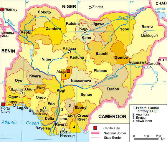

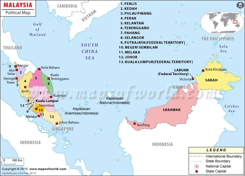


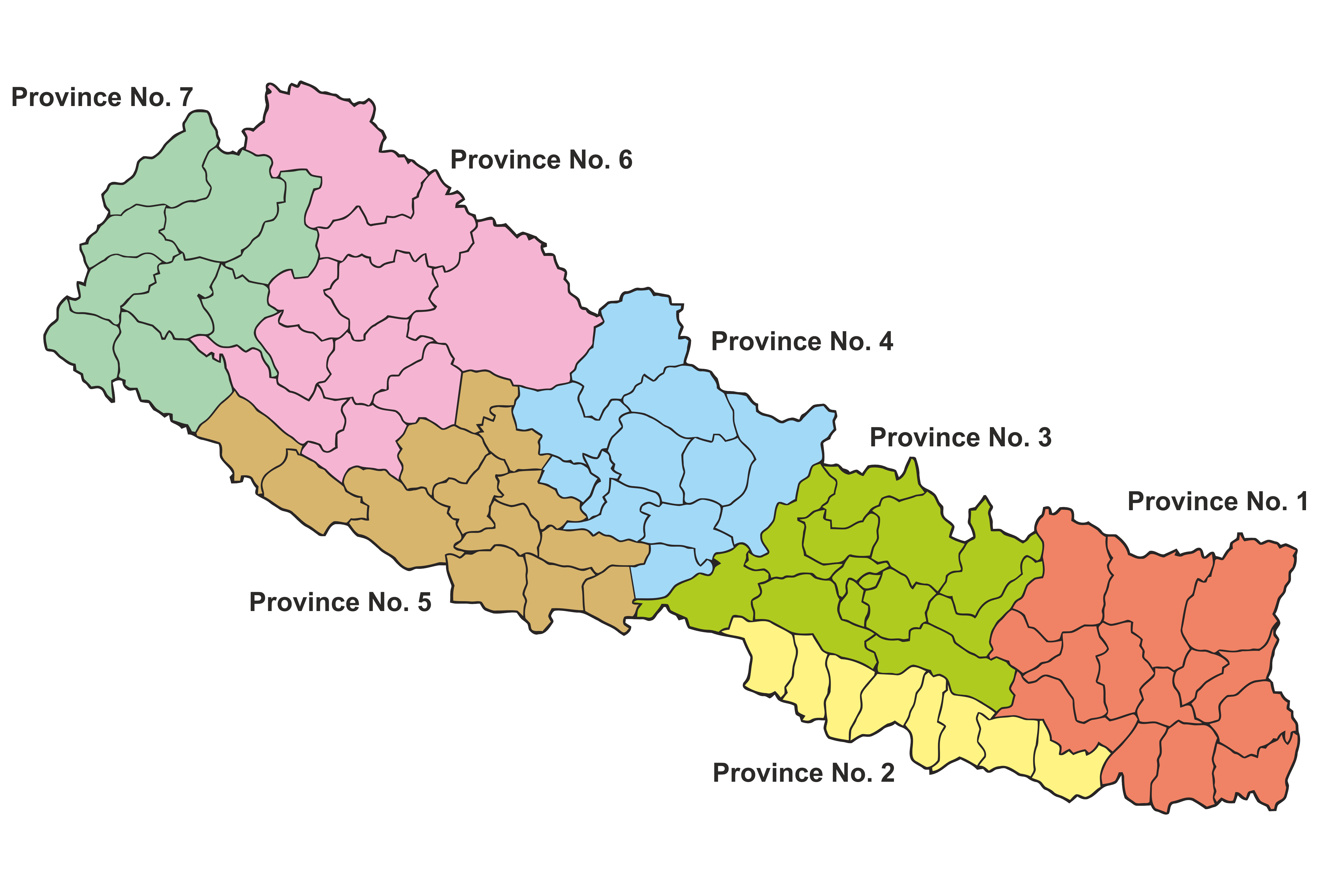


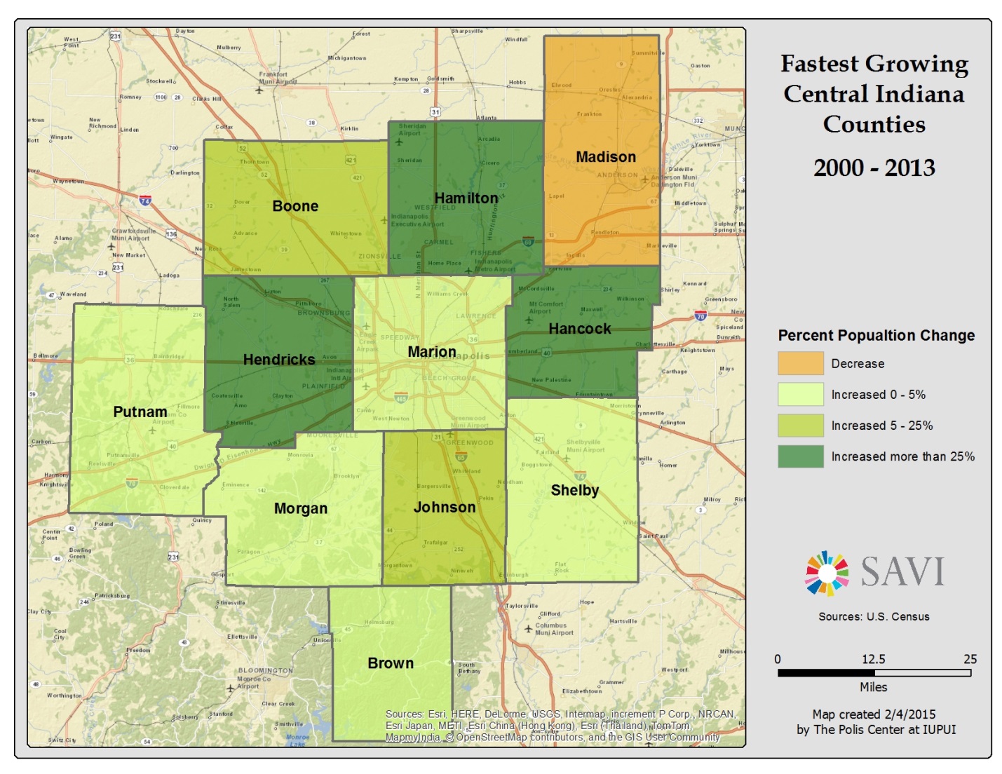
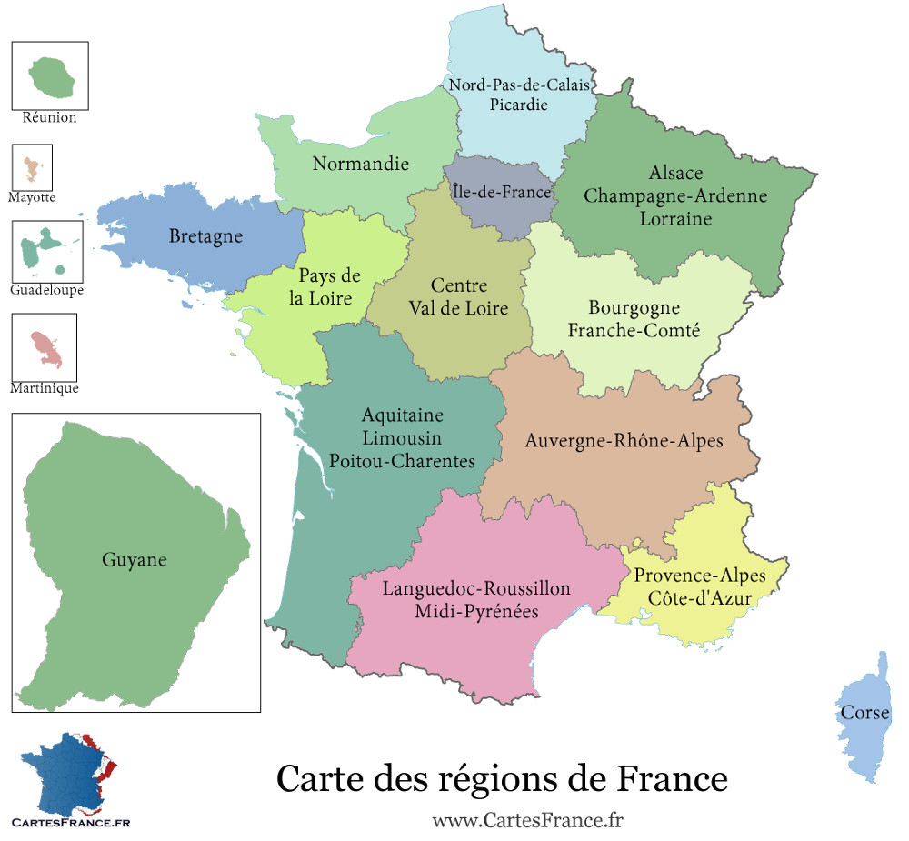


