Code Monkey home page Code Monkey logo

bayesloop's Introduction

bayesloop

Build status Documentation status Coverage Status License: MIT DOI

Time series analysis today is an important cornerstone of quantitative science in many disciplines, including natural and life sciences as well as economics and social sciences. Regarding diverse phenomena like tumor cell migration, brain activity and stock trading, a similarity of these complex systems becomes apparent: the observable data we measure – cell migration paths, neuron spike rates and stock prices – are the result of a multitude of underlying processes that act over a broad range of spatial and temporal scales. It is thus to expect that the statistical properties of these systems are not constant, but themselves show stochastic or deterministic dynamics of their own. Time series models used to understand the dynamics of complex systems therefore have to account for temporal changes of the models' parameters.

bayesloop is a python module that focuses on fitting time series models with time-varying parameters and model selection based on Bayesian inference. Instead of relying on MCMC methods, bayesloop uses a grid-based approach to evaluate probability distributions, allowing for an efficient approximation of the marginal likelihood (evidence). The marginal likelihood represents a powerful tool to objectively compare different models and/or optimize the hyper-parameters of hierarchical models. To avoid the curse of dimensionality when analyzing time series models with time-varying parameters, bayesloop employs a sequential inference algorithm that is based on the forward-backward-algorithm used in Hidden Markov models. Here, the relevant parameter spaces are kept low-dimensional by processing time series data step by step. The module covers a large class of time series models and is easily extensible.

bayesloop has been successfully employed in cancer research (studying the migration paths of invasive tumor cells), financial risk assessment, climate research and accident analysis. For a detailed description of these applications, see the following articles:

Bayesian model selection for complex dynamic systems
Mark C., Metzner C., Lautscham L., Strissel P.L., Strick R. and Fabry B.
Nature Communications 9:1803 (2018)

Superstatistical analysis and modelling of heterogeneous random walks
Metzner C., Mark C., Steinwachs J., Lautscham L., Stadler F. and Fabry B.
Nature Communications 6:7516 (2015)

Features

  • infer time-varying parameters from time series data
  • compare hypotheses about parameter dynamics (model evidence)
  • create custom models based on SymPy and SciPy
  • straight-forward handling of missing data points
  • predict future parameter values
  • detect change-points and structural breaks in time series data
  • employ model selection to online data streams

Getting started

For a comprehensive introduction and overview of the main features that bayesloop provides, see the documentation.

The following code provides a minimal example of an analysis carried out using bayesloop. The data here consists of the number of coal mining disasters in the UK per year from 1851 to 1962 (see this article for further information).

import bayesloop as bl
import matplotlib.pyplot as plt
import seaborn as sns

S = bl.HyperStudy()  # start new data study
S.loadExampleData()  # load data array

# observed number of disasters is modeled by Poisson distribution
L = bl.om.Poisson('rate')

# disaster rate itself may change gradually over time
T = bl.tm.GaussianRandomWalk('sigma', bl.cint(0, 1.0, 20), target='rate')

S.set(L, T)
S.fit()  # inference

# plot data together with inferred parameter evolution
plt.figure(figsize=(8, 3))

plt.subplot2grid((1, 3), (0, 0), colspan=2)
plt.xlim([1852, 1961])
plt.bar(S.rawTimestamps, S.rawData, align='center', facecolor='r', alpha=.5)
S.plot('rate')
plt.xlabel('year')

# plot hyper-parameter distribution
plt.subplot2grid((1, 3), (0, 2))
plt.xlim([0, 1])
S.plot('sigma', facecolor='g', alpha=0.7, lw=1, edgecolor='k')
plt.tight_layout()
plt.show()

Analysis plot

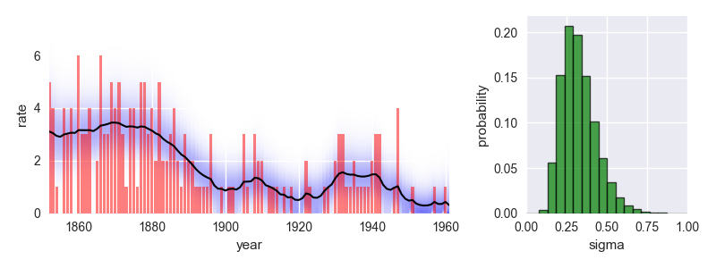
This analysis indicates a significant improvement of safety conditions between 1880 and 1900. Check out the documentation for further insights!

Installation

The easiest way to install the latest release version of bayesloop is via pip:

pip install bayesloop

Alternatively, a zipped version can be downloaded here. The module is installed by calling python setup.py install.

Development version

The latest development version of bayesloop can be installed from the master branch using pip (requires git):

pip install git+https://github.com/christophmark/bayesloop

Alternatively, use this zipped version or clone the repository.

Dependencies

bayesloop is tested on Python 3.8. It depends on NumPy, SciPy, SymPy, matplotlib, tqdm and cloudpickle. All except the last two are already included in the Anaconda distribution of Python. Windows users may also take advantage of pre-compiled binaries for all dependencies, which can be found at Christoph Gohlke's page.

Optional dependencies

bayesloop supports multiprocessing for computationally expensive analyses, based on the pathos module. The latest version can be obtained directly from GitHub using pip (requires git):

pip install git+https://github.com/uqfoundation/pathos

Note: Windows users need to install a C compiler before installing pathos. One possible solution for 64bit systems is to install Microsoft Visual C++ 2008 SP1 Redistributable Package (x64) and Microsoft Visual C++ Compiler for Python 2.7.

License

The MIT License (MIT)

If you have any further questions, suggestions or comments, do not hesitate to contact me: [email protected]

bayesloop's People

Contributors

christophmark avatar dependabot[bot] avatar ezzeddin avatar

Stargazers

 avatar  avatar  avatar  avatar  avatar  avatar  avatar  avatar  avatar  avatar  avatar  avatar  avatar  avatar  avatar  avatar  avatar  avatar  avatar  avatar  avatar  avatar  avatar  avatar  avatar  avatar  avatar  avatar  avatar  avatar  avatar  avatar  avatar  avatar  avatar  avatar  avatar  avatar  avatar  avatar  avatar  avatar  avatar  avatar  avatar  avatar  avatar  avatar  avatar  avatar  avatar  avatar  avatar  avatar  avatar  avatar  avatar  avatar  avatar  avatar  avatar  avatar  avatar  avatar  avatar  avatar  avatar  avatar  avatar  avatar  avatar  avatar  avatar  avatar  avatar  avatar  avatar  avatar  avatar  avatar  avatar  avatar  avatar  avatar  avatar  avatar  avatar  avatar  avatar  avatar  avatar  avatar  avatar  avatar  avatar  avatar  avatar  avatar  avatar  avatar

Watchers

 avatar  avatar  avatar  avatar  avatar  avatar  avatar  avatar  avatar  avatar  avatar  avatar  avatar

bayesloop's Issues

Add linear regression model

Observation model like the AR1, but with a constant instead of the auto-correlation term. This allows to independent Gaussian noise with non-zero mean, or, in the case that first order data differences of data points are provided, basic linear regression (with static transition model). Further, this approach also allows to identify trends dynamically (with other transition models). Especially the case of abrupt on/off-sets (regime-switching process) of trends might yield new insights into some systems...

Serial transition model

In some applications, different transition models apply for different time segments. Therefore, a concept similar to the combined transition model would be desirable that e.g. assumes static parameters until a certain time step t, and after that assumes Gaussian fluctuations.

Test failing, possibly because of changes to scipy optimize (?)

See here:

=================================== FAILURES ===================================
_____________________ TestTwoParameterModel.test_optimize ______________________
self = <test_study.TestTwoParameterModel object at 0x7fa2fc813610>
    def test_optimize(self):
        # carry out fit
        S = bl.Study()
        S.loadData(np.array([1, 2, 3, 4, 5]))
        S.setOM(bl.om.Gaussian('mean', bl.cint(0, 6, 20), 'sigma', bl.oint(0, 2, 20), prior=lambda m, s: 1/s**3))
        T = bl.tm.CombinedTransitionModel(bl.tm.GaussianRandomWalk('sigma', 1.07, target='mean'),
                                          bl.tm.RegimeSwitch('log10pMin', -3.90))
        S.setTM(T)
        S.optimize()
        # test parameter distributions
>       np.testing.assert_allclose(S.getParameterDistributions('mean', density=False)[1][:, 5],
                                   [4.525547e-04, 1.677968e-03, 2.946498e-07, 1.499508e-08, 1.102637e-09],
                                   rtol=1e-05, err_msg='Erroneous posterior distribution values.')
E       AssertionError: 
E       Not equal to tolerance rtol=1e-05, atol=0
E       Erroneous posterior distribution values.
E       Mismatched elements: 5 / 5 (100%)
E       Max absolute difference: 6.48028681e-08
E       Max relative difference: 0.00072859
E        x: array([4.525729e-04, 1.677903e-03, 2.945258e-07, 1.498415e-08,
E              1.102384e-09])
E        y: array([4.525547e-04, 1.677968e-03, 2.946498e-07, 1.499508e-08,
E              1.102637e-09])
test_study.py:330: AssertionError
----------------------------- Captured stdout call -----------------------------
+ Created new study.
+ Successfully imported array.
+ Observation model: Gaussian observations. Parameter(s): ['mean', 'sigma']
+ Transition model: Combined transition model. Hyper-Parameter(s): ['sigma', 'log10pMin']
+ Starting optimization...
  --> All model parameters are optimized (except change/break-points).
    + Log10-evidence: -3.47897 - Parameter values: [ 1.07 -3.9 ]
    + Log10-evidence: -3.75097 - Parameter values: [ 2.07 -3.9 ]
    + Log10-evidence: -3.48400 - Parameter values: [ 1.07 -2.9 ]
    + Log10-evidence: -6.94856 - Parameter values: [ 0.07017134 -3.91851083]
    + Log10-evidence: -4.399[24](https://github.com/christophmark/bayesloop/runs/7068584434?check_suite_focus=true#step:5:25) - Parameter values: [ 0.57008567 -3.909[25](https://github.com/christophmark/bayesloop/runs/7068584434?check_suite_focus=true#step:5:26)542]
    + Log10-evidence: -3.52186 - Parameter values: [ 1.31999906 -3.90068388]
    + Log10-evidence: -3.47888 - Parameter values: [ 1.06965806 -4.02499953]
    + Log10-evidence: -3.59705 - Parameter values: [ 0.81965823 -4.02529235]
    + Log10-evidence: -3.49207 - Parameter values: [ 1.19465698 -4.02551875]
    + Log10-evidence: -3.48383 - Parameter values: [ 1.00715847 -4.02522561]
    + Log10-evidence: -3.47981 - Parameter values: [ 1.1009061  -4.02534994]
    + Log10-evidence: -3.47888 - Parameter values: [ 1.06948286 -4.04062355]
    + Log10-evidence: -3.48005 - Parameter values: [ 1.03823334 -4.04079793]
    + Log10-evidence: -3.47909 - Parameter values: [ 1.08510319 -4.04100528]
    + Log10-evidence: -3.47890 - Parameter values: [ 1.06167279 -4.04081835]
    + Log10-evidence: -3.47888 - Parameter values: [ 1.07332013 -4.04135437]
    + Log10-evidence: -3.47888 - Parameter values: [ 1.06911745 -4.04254219]
    + Log10-evidence: -3.47883 - Parameter values: [ 1.06570473 -4.0396313 ]
    + Log10-evidence: -3.47889 - Parameter values: [ 1.06187307 -4.03887159]
    + Log10-evidence: -3.47889 - Parameter values: [ 1.06666122 -4.03792841]
    + Log10-evidence: -3.47890 - Parameter values: [ 1.06608651 -4.04154675]
    + Log10-evidence: -3.47884 - Parameter values: [ 1.0647419  -4.03946811]
    + Log10-evidence: -3.47883 - Parameter values: [ 1.06578141 -4.04011352]
    + Log10-evidence: -3.47890 - Parameter values: [ 1.06602252 -4.04007519]
    + Log10-evidence: -3.47884 - Parameter values: [ 1.06529985 -4.0401943 ]
    + Log10-evidence: -3.47890 - Parameter values: [ 1.06602539 -4.04012232]
    + Log10-evidence: -3.47883 - Parameter values: [ 1.06568278 -4.04013005]
    + Log10-evidence: -3.47890 - Parameter values: [ 1.06578967 -4.04016284]
    + Log10-evidence: -3.47883 - Parameter values: [ 1.0657657  -4.04001477]
+ Finished optimization.
+ Started new fit:
    + Formatted data.
    + Set prior (function): <lambda>. Values have been re-normalized.
    + Finished forward pass.
    + Log10-evidence: -3.47883
    + Finished backward pass.
    + Computed mean parameter values.
----------------------------- Captured stderr call -----------------------------
  0%|          | 0/5 [00:00<?, ?it/s]
100%|██████████| 5/5 [00:00<00:00, 6[26](https://github.com/christophmark/bayesloop/runs/7068584434?check_suite_focus=true#step:5:27)0.16it/s]
  0%|          | 0/5 [00:00<?, ?it/s]
100%|██████████| 5/5 [00:00<00:00, 51[32](https://github.com/christophmark/bayesloop/runs/7068584434?check_suite_focus=true#step:5:33).[53](https://github.com/christophmark/bayesloop/runs/7068584434?check_suite_focus=true#step:5:54)it/s]
=============================== warnings summary ===============================
../../../../../../opt/hostedtoolcache/Python/3.8.12/x[64](https://github.com/christophmark/bayesloop/runs/7068584434?check_suite_focus=true#step:5:65)/lib/python3.8/site-packages/bayesloop/core.py:23
  /opt/hostedtoolcache/Python/3.8.12/x64/lib/python3.8/site-packages/bayesloop/core.py:23: DeprecationWarning: Using or importing the ABCs from 'collections' instead of from 'collections.abc' is deprecated since Python 3.3, and in 3.10 it will stop working
    from collections import OrderedDict, Iterable
../../../../../../opt/hostedtoolcache/Python/3.8.12/x64/lib/python3.8/site-packages/bayesloop/transitionModels.py:15
  /opt/hostedtoolcache/Python/3.8.12/x64/lib/python3.8/site-packages/bayesloop/transitionModels.py:15: DeprecationWarning: Please use `gaussian_filter1d` from the `scipy.ndimage` namespace, the `scipy.ndimage.filters` namespace is deprecated.
    from scipy.ndimage.filters import gaussian_filter1d
../../../../../../opt/hostedtoolcache/Python/3.8.12/x64/lib/python3.8/site-packages/bayesloop/transitionModels.py:16
  /opt/hostedtoolcache/Python/3.8.12/x64/lib/python3.8/site-packages/bayesloop/transitionModels.py:16: DeprecationWarning: Please use `shift` from the `scipy.ndimage` namespace, the `scipy.ndimage.interpolation` namespace is deprecated.
    from scipy.ndimage.interpolation import shift

Check if marginal likelihood computation is suited to compare models with different structure.

Test case could be a simulated AR-1 process with correlation coeff. equal to zero. This data can be analyzed with static parameters (no real transition model), but with two observation models: the AR-1 process that features two parameters, or the more simple Gaussian random walk with only one parameter. In the limit of infinite data points, the marginal likelihoods should converge to the same value. If not, we need to account for different discretization of the parameter spaces.

Implement raster-study

Up to this point, only the change-point study allows to determine the distribution of hyper-parameter values (change-point distribution). A similar study could be performed with continuous hyper-parameters by choosing discrete values on a grid to approximate the distribution of those hyper-parameters. The current change-point study can probably be integrated in this more general scheme.

Prior distributions

While bayesloop allows to set prior distributions at some stages in the modeling process, the main inference algorithm of the study class still assumes a flat prior.

Prior distributions could be implemented based on scipy.stats.

Uninformative priors could be implemented directly into the observation models.

Add support for OnlineStudy in probability parser submodule

The current version of the probability parser (52372c7) only supports Study, HyperStudy and ChangepointStudy instances. Implementation is probably not trivial as hyper-parameters are assumed to be time-independent in the current version, while OnlineStudy instances support time-varying hyper-parameters.

SymPy observation model tests fail for Python 3.5

A fit using a 2-parameter SymPy observation model on Python 3.5 results in an erroneous log-evidence of -inf (detected by Travis CI). The problem seems to be version-specific as the tests pass on both Python 2.7 and 3.6.

Introduce checks for analysis work-flow

Currently, no checks are performed to ensure all parameters are set before a fitting method is called. Also, the default gridsize and parameter boundaries are set but not used.

'dict_keys' object has no attribute 'index' error when following 'Anomalous diffusion' example in docs

Hello, I'm using python 3.6.5 and I get the following error when trying to run through the Anomalous diffusion example:

.../bayesloop/transitionModels.py in computeForwardPrior(self, posterior, t)
    100             ndarray: Prior parameter distribution for subsequent time step
    101         """
--> 102         axisToTransform = self.study.observationModel.parameterNames.index(self.selectedParameter)
    103         normedSigma = self.hyperParameterValues[0]/self.latticeConstant[axisToTransform]
    104 

AttributeError: 'dict_keys' object has no attribute 'index'

The line of code in the example:
L = bl.om.SymPy(normal, {'D': bl.oint(0, 15, 5000)})

Should be changed to:
L = bl.om.SymPy(normal, 'D', bl.oint(0, 15, 5000))

Unless you want to deal with version issues for indexing dict_keys.

Loading data as list fails

Loading data as a numpy-array works fine, but using a "standard" Python list results in an error. The error occurs because the movingWindow function during data preprocessing expects a numpy array.

No defined order of parameters in SymPy/SciPy models

The values of observation model parameters in SymPy/SciPy models are defined via a dictionary. As dictionaries are not ordered, one has to look up the order of the parameters in the attribute parameterNames of the observation model instance. Without knowing the order, defining prior distributions can result in a mixup of the parameters and inference may fail or produce unintended results!

Arbitrary deterministic transition models

Any kind of Python function may serve as a determinsitic transition model (like the Linear model already implemented). All the requirements for this should be present in the current code.

Apply seaborn styling only "locally"

Currently, bayesloop changes plotting behavior by importing seaborn. However, seaborn styling should only apply to plots created by bayesloop-functions and should not apply to other plots created by a script that imports bayesloop.

Add custom time stamps to data

Up to this point, time steps in bayesloop start at 0 and are incremented by one for each data point. It would be much more natural to provide custom time stamps (e.g. years). This can probably be directly implemented into the loadData method.

Add online study class

Instead of using forwardOnly with common fit-method, an "update" method would only take the new incoming data point and update the parameter distribution. The length of the history for distributions and mean parameter values can be chosen.

Simpler implementation of new observation models

Creating new observation models requires a lot of knowledge of how bayesloop works. By creating a parent class for observation models that takes care of integrating the whole grid-stuff and missing value routines, we could probably create observation models from any scipy.stats object on-the-fly.

Get number positivity

I have a rule that throws numbers between -50 and 50 randomly, is there any way to predict the sign (positive or negative) of the next release with at least 90% accuracy based on a historical record?

Performance

Hi,

I am following along the example:

for r in tqdm_notebook(logReturns):
    S.step(r)

It is taking about 1.5 seconds for each step to process. Is this normal or did I do something wrong? I have minute data and about 1M prices of historical data. Would I need to send all of them into the step function? I am sorry but I am new to probabilistic programming and bayesloop. Thanks for any help/guidance.

bayesloop module fails to load, pythin 3.7.7 64-bit

I wanted to try out the bayesloop. I followed the installation instructions in the documentation, but module import failed:

Python 3.7.7 (default, May  6 2020, 11:45:54) [MSC v.1916 64 bit (AMD64)] :: Anaconda, Inc. on win32
Type "help", "copyright", "credits" or "license" for more information.
>>> import bayesloop
Traceback (most recent call last):
  File "<stdin>", line 1, in <module>
  File "D:\workspace\tools\Miniconda3\lib\site-packages\bayesloop\__init__.py", line 4, in <module>
    from .core import Study, HyperStudy, ChangepointStudy, OnlineStudy
  File "D:\workspace\tools\Miniconda3\lib\site-packages\bayesloop\core.py", line 15, in <module>
    from scipy.misc import factorial
ImportError: cannot import name 'factorial' from 'scipy.misc' (D:\workspace\tools\Miniconda3\lib\site-packages\scipy\misc\__init__.py)

I tried to resolve the problem, following https://stackoverflow.com/questions/56283294/importerror-cannot-import-name-factorial but that didn't resolve.

Any idea on how to overcome this issue?

Optimization of Hyperparameters

Create a new study-class that optimizes the hyperparameters of a transition model using some optimization algo that does not depend on gradient information (Powell or Nelder-Mead). May require to reimplement the way hyperparameters are stored within the transition models (maybe use a dictionary to access the names of the parameters...).

Recommend Projects

  • React photo React

    A declarative, efficient, and flexible JavaScript library for building user interfaces.

  • Vue.js photo Vue.js

    🖖 Vue.js is a progressive, incrementally-adoptable JavaScript framework for building UI on the web.

  • Typescript photo Typescript

    TypeScript is a superset of JavaScript that compiles to clean JavaScript output.

  • TensorFlow photo TensorFlow

    An Open Source Machine Learning Framework for Everyone

  • Django photo Django

    The Web framework for perfectionists with deadlines.

  • D3 photo D3

    Bring data to life with SVG, Canvas and HTML. 📊📈🎉

Recommend Topics

  • javascript

    JavaScript (JS) is a lightweight interpreted programming language with first-class functions.

  • web

    Some thing interesting about web. New door for the world.

  • server

    A server is a program made to process requests and deliver data to clients.

  • Machine learning

    Machine learning is a way of modeling and interpreting data that allows a piece of software to respond intelligently.

  • Game

    Some thing interesting about game, make everyone happy.

Recommend Org

  • Facebook photo Facebook

    We are working to build community through open source technology. NB: members must have two-factor auth.

  • Microsoft photo Microsoft

    Open source projects and samples from Microsoft.

  • Google photo Google

    Google ❤️ Open Source for everyone.

  • D3 photo D3

    Data-Driven Documents codes.