SmallPebble

SmallPebble is a minimal automatic differentiation and deep learning library written from scratch in Python, using NumPy/CuPy.

The implementation is relatively small, and mainly in the file: smallpebble.py. To help understand it, check out this introduction to autodiff, which presents an autodiff framework that works in the same way as SmallPebble (except using scalars instead of NumPy arrays).

SmallPebble's raison d'etre is to be a simplified deep learning implementation, for those who want to learn what’s under the hood of deep learning frameworks. However, because it is written in terms of vectorised NumPy/CuPy operations, it performs well enough for non-trivial models to be trained using it.

The name SmallPebble is a reference to the Latin translation of 'calculus', which is ‘pebble’.

Highlights

Relatively simple implementation.
Can run on GPU, using CuPy.
Various operations, such as matmul, conv2d, maxpool2d.
Array broadcasting support.
Eager or lazy execution.
Powerful API for creating models.
It's easy to add new SmallPebble functions.

Notes

Graphs are built implicitly via Python objects referencing Python objects. When get_gradients is called, autodiff is carried out on the whole sub-graph. The default array library is NumPy.

Read on to see:

Example models created and trained using SmallPebble.
A brief guide to using SmallPebble.

import matplotlib.pyplot as plt
import numpy as np
from tqdm.notebook import tqdm
import smallpebble as sp
from smallpebble.misc import load_data

Training a neural network to classify handwritten digits (MNIST)

"Load the dataset, and create a validation set."

X_train, y_train, _, _ = load_data('mnist')  # load / download from openml.org
X_train = X_train/255  # normalize

# Seperate out data for validation.
X = X_train[:50_000, ...]
y = y_train[:50_000]
X_eval = X_train[50_000:60_000, ...]
y_eval = y_train[50_000:60_000]

"Plot, to check we have the right data."

plt.figure(figsize=(5,5))
for i in range(25):
    plt.subplot(5,5,i+1)
    plt.xticks([])
    plt.yticks([])
    plt.grid(False)
    plt.imshow(X_train[i,:].reshape(28,28), cmap='gray', vmin=0, vmax=1)

plt.show()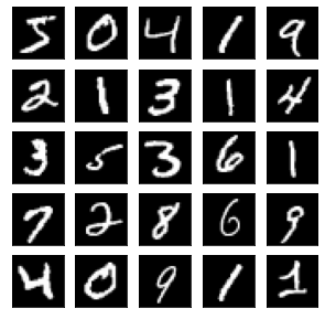

"Create a model, with two fully connected hidden layers."

X_in = sp.Placeholder()
y_true = sp.Placeholder()

h = sp.linearlayer(28*28, 100)(X_in)
h = sp.Lazy(sp.leaky_relu)(h)
h = sp.linearlayer(100, 100)(h)
h = sp.Lazy(sp.leaky_relu)(h)
h = sp.linearlayer(100, 10)(h)
y_pred = sp.Lazy(sp.softmax)(h)
loss = sp.Lazy(sp.cross_entropy)(y_pred, y_true)

learnables = sp.get_learnables(y_pred)

loss_vals = []
validation_acc = []

"Train model, while measuring performance on the validation dataset."

NUM_ITERS = 300
BATCH_SIZE = 200

eval_batch = sp.batch(X_eval, y_eval, BATCH_SIZE)
adam = sp.Adam()  # Adam optimization

for i, (xbatch, ybatch) in tqdm(enumerate(sp.batch(X, y, BATCH_SIZE)), total=NUM_ITERS):
    if i >= NUM_ITERS: break
    
    X_in.assign_value(sp.Variable(xbatch))
    y_true.assign_value(ybatch)
    
    loss_val = loss.run()  # run the graph
    if np.isnan(loss_val.array):
        print("loss is nan, aborting.")
        break
    loss_vals.append(loss_val.array)
        
    # Compute gradients, and use to carry out learning step:
    gradients = sp.get_gradients(loss_val)
    adam.training_step(learnables, gradients)
        
    # Compute validation accuracy:
    x_eval_batch, y_eval_batch = next(eval_batch)
    X_in.assign_value(sp.Variable(x_eval_batch))
    predictions = y_pred.run()
    predictions = np.argmax(predictions.array, axis=1)
    accuracy = (y_eval_batch == predictions).mean()
    validation_acc.append(accuracy)

# Plot results:
print(f'Final validation accuracy: {np.mean(validation_acc[-10:]):.4f}')
plt.figure(figsize=(14, 4))
plt.subplot(1, 2, 1)
plt.ylabel('Loss')
plt.xlabel('Iteration')
plt.plot(loss_vals)
plt.subplot(1, 2, 2)
plt.ylabel('Validation accuracy')
plt.xlabel('Iteration')
plt.suptitle('Neural network trained on MNIST, using SmallPebble.')
plt.ylim([0, 1])
plt.plot(validation_acc)
plt.show()

Final validation accuracy: 0.9290

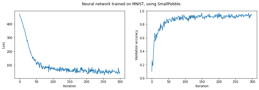
Training a convolutional neural network on CIFAR-10, using CuPy

This was run on Google Colab, with a GPU.

"Load the CIFAR dataset."

X_train, y_train, _, _ = load_data('cifar')  # load/download from openml.org
X_train = X_train/255  # normalize

"""Plot, to check it's the right data.

(This cell's code is from: https://www.tensorflow.org/tutorials/images/cnn#verify_the_data)
"""

class_names = ['airplane', 'automobile', 'bird', 'cat', 'deer',
               'dog', 'frog', 'horse', 'ship', 'truck']

plt.figure(figsize=(8,8))
for i in range(25):
    plt.subplot(5,5,i+1)
    plt.xticks([])
    plt.yticks([])
    plt.grid(False)
    plt.imshow(X_train[i,:].reshape(32,32,3))
    plt.xlabel(class_names[y_train[i]])

plt.show()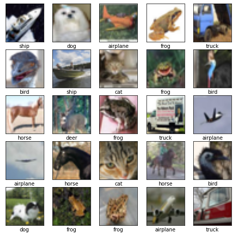

"Switch array library to CuPy, so can use GPU."

import cupy

sp.use(cupy)

print(sp.array_library.library.__name__)  # should be 'cupy'

cupy

"Convert data to CuPy arrays"

X_train = cupy.array(X_train)
y_train = cupy.array(y_train)

# Seperate out data for validation as before.
X = X_train[:45_000, ...]
y = y_train[:45_000]
X_eval = X_train[45_000:50_000, ...]
y_eval = y_train[45_000:50_000]

"""Define a model."""

X_in = sp.Placeholder()
y_true = sp.Placeholder()

h = sp.convlayer(height=3, width=3, depth=3, n_kernels=64, padding='VALID')(X_in)
h = sp.Lazy(sp.leaky_relu)(h)
h = sp.Lazy(lambda a: sp.maxpool2d(a, 2, 2, strides=[2, 2]))(h)

h = sp.convlayer(3, 3, 64, 128, padding='VALID')(h)
h = sp.Lazy(sp.leaky_relu)(h)
h = sp.Lazy(lambda a: sp.maxpool2d(a, 2, 2, strides=[2, 2]))(h)

h = sp.convlayer(3, 3, 128, 128, padding='VALID')(h)
h = sp.Lazy(sp.leaky_relu)(h)
h = sp.Lazy(lambda a: sp.maxpool2d(a, 2, 2, strides=[2, 2]))(h)

h = sp.Lazy(lambda x: sp.reshape(x, [-1, 3*3*128]))(h)
h = sp.linearlayer(3*3*128, 512)(h)
h = sp.Lazy(sp.leaky_relu)(h)

h = sp.linearlayer(512, 10)(h)
h = sp.Lazy(sp.softmax)(h)

y_pred = h
loss = sp.Lazy(sp.cross_entropy)(y_pred, y_true)

learnables = sp.get_learnables(y_pred)

loss_vals = []
validation_acc = []

# Check we get the expected dimensions
X_in.assign_value(sp.Variable(X[0:3, :].reshape([-1, 32, 32, 3])))
h.run().shape

(3, 10)

Train the model.

NUM_ITERS = 3000
BATCH_SIZE = 128

eval_batch = sp.batch(X_eval, y_eval, BATCH_SIZE)
adam = sp.Adam()

for i, (xbatch, ybatch) in tqdm(enumerate(sp.batch(X, y, BATCH_SIZE)), total=NUM_ITERS):
    if i >= NUM_ITERS: break
       
    xbatch_images = xbatch.reshape([-1, 32, 32, 3])
    X_in.assign_value(sp.Variable(xbatch_images))
    y_true.assign_value(ybatch)
    
    loss_val = loss.run()
    if np.isnan(loss_val.array):
        print("Aborting, loss is nan.")
        break
    loss_vals.append(loss_val.array)
    
    # Compute gradients, and carry out learning step.
    gradients = sp.get_gradients(loss_val)  
    adam.training_step(learnables, gradients)
    
    # Compute validation accuracy:
    x_eval_batch, y_eval_batch = next(eval_batch)
    X_in.assign_value(sp.Variable(x_eval_batch.reshape([-1, 32, 32, 3])))
    predictions = y_pred.run()
    predictions = np.argmax(predictions.array, axis=1)
    accuracy = (y_eval_batch == predictions).mean()
    validation_acc.append(accuracy)

print(f'Final validation accuracy: {np.mean(validation_acc[-10:]):.4f}')
plt.figure(figsize=(14, 4))
plt.subplot(1, 2, 1)
plt.ylabel('Loss')
plt.xlabel('Iteration')
plt.plot(loss_vals)
plt.subplot(1, 2, 2)
plt.ylabel('Validation accuracy')
plt.xlabel('Iteration')
plt.suptitle('CNN trained on CIFAR-10, using SmallPebble.')
plt.ylim([0, 1])
plt.plot(validation_acc)
plt.show()

Final validation accuracy: 0.7273

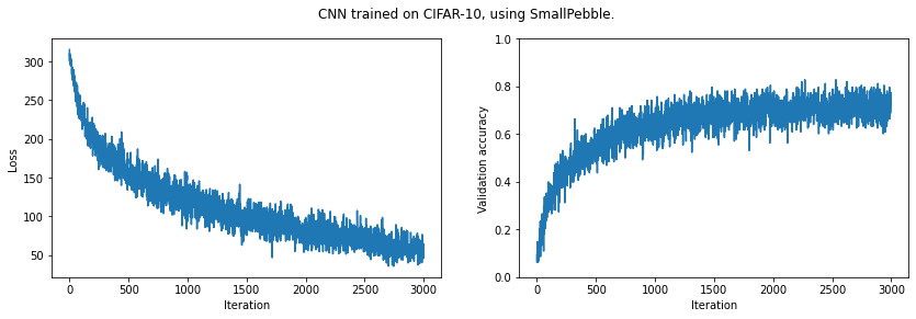
It looks like we could improve our results by training for longer. (And of course we could improve our model architecture.)

Brief guide to using SmallPebble

SmallPebble provides the following building blocks to make models with:

sp.Variable
Operations, such as sp.add, sp.mul, etc.
sp.get_gradients
sp.Lazy
sp.Placeholder (this is really just sp.Lazy on the identity function)
sp.learnable
sp.get_learnables

The following examples show how these are used.

Switching between NumPy and CuPy

We can dynamically switch between NumPy and CuPy. (Assuming you have a CuPy compatible GPU and CuPy set up. Note, CuPy is available on Google Colab, if you change the runtime to GPU.)

import cupy
import numpy
import smallpebble as sp
 
# Switch to CuPy
sp.use(cupy)
print(sp.array_library.library.__name__)  # should be 'cupy'

# Switch back to NumPy:
sp.use(numpy)
print(sp.array_library.library.__name__)  # should be 'numpy'

cupy
numpy

sp.Variable & sp.get_gradients

With SmallPebble, you can:

Wrap NumPy arrays in sp.Variable
Apply SmallPebble operations (e.g. sp.matmul, sp.add, etc.)
Compute gradients with sp.get_gradients

a = sp.Variable(np.random.random([2, 2]))
b = sp.Variable(np.random.random([2, 2]))
c = sp.Variable(np.random.random([2]))
y = sp.mul(a, b) + c
print('y.array:\n', y.array)

gradients = sp.get_gradients(y)
grad_a = gradients[a]
grad_b = gradients[b]
grad_c = gradients[c]
print('grad_a:\n', grad_a)
print('grad_b:\n', grad_b)
print('grad_c:\n', grad_c)

y.array:
 [[0.10193547 0.94806202]
 [0.3119681  1.04487129]]
grad_a:
 [[0.02006619 0.66175381]
 [0.23060704 0.80155288]]
grad_b:
 [[0.94073311 0.6947422 ]
 [0.99263909 0.69434916]]
grad_c:
 [2. 2.]

Note that y is computed straight away, i.e. the (forward) computation happens immediately.

Also note that y is a sp.Variable and we could continue to carry out SmallPebble operations on it.

sp.Lazy & sp.Placeholder

Lazy graphs are constructed using sp.Lazy and sp.Placeholder.

lazy_node = sp.Lazy(lambda a, b: a + b)(1, 2)
print(lazy_node)
print(lazy_node.run())

<smallpebble.smallpebble.Lazy object at 0x7f7cc5ee7ad0>
3

a = sp.Lazy(lambda a: a)(2)
y = sp.Lazy(lambda a, b, c: a * b + c)(a, 3, 4)
print(y)
print(y.run())

<smallpebble.smallpebble.Lazy object at 0x7f7cc5f03990>
10

Forward computation does not happen immediately - only when .run() is called.

a = sp.Placeholder()
b = sp.Variable(np.random.random([2, 2]))
y = sp.Lazy(sp.matmul)(a, b)

a.assign_value(sp.Variable(np.array([[1,2], [3,4]])))

result = y.run()
print('result.array:\n', result.array)

result.array:
 [[1.25794861 1.84124373]
 [3.01624003 3.89064526]]

You can use .run() as many times as you like.

Let's change the placeholder value and re-run the graph:

a.assign_value(sp.Variable(np.array([[10,20], [30,40]])))
result = y.run()
print('result.array:\n', result.array)

result.array:
 [[12.57948615 18.41243733]
 [30.16240033 38.90645264]]

Finally, let's compute gradients:

gradients = sp.get_gradients(result)

Note that sp.get_gradients is called on result, which is a sp.Variable, not on y, which is a sp.Lazy instance.

sp.learnable & sp.get_learnables

Use sp.learnable to flag parameters as learnable, allowing them to be extracted from a lazy graph with sp.get_learnables.

This enables a workflow of: building a model, while flagging parameters as learnable, and then extracting all the parameters in one go at the end.

a = sp.Placeholder()
b = sp.learnable(sp.Variable(np.random.random([2, 1])))
y = sp.Lazy(sp.matmul)(a, b)
y = sp.Lazy(sp.add)(y, sp.learnable(sp.Variable(np.array([5]))))

learnables = sp.get_learnables(y)

for learnable in learnables:
    print(learnable)

<smallpebble.smallpebble.Variable object at 0x7f7cc5ede410>
<smallpebble.smallpebble.Variable object at 0x7f7cc5ede5d0>

sradc / smallpebble Goto Github PK

smallpebble's Introduction

SmallPebble

Training a neural network to classify handwritten digits (MNIST)

Training a convolutional neural network on CIFAR-10, using CuPy

Brief guide to using SmallPebble

Switching between NumPy and CuPy

sp.Variable & sp.get_gradients

sp.Lazy & sp.Placeholder

sp.learnable & sp.get_learnables

smallpebble's People

Contributors

Stargazers

Watchers

Forkers

smallpebble's Issues

Recommend Projects

Recommend Topics

Recommend Org