- 针对单个样本的解决方案
- 针对肿瘤N-T配对样本的解决方案
- 针对多个样本的解决方案
在bioconductor上面看到一个R包 seqCNA:
读其文档的时候发现,是可以针对单个样本进行拷贝数变异分析的,代码如下:
library(seqCNA)
data(seqsumm_HCC1143)
head(seqsumm_HCC1143)
dim(seqsumm_HCC1143)
tail(seqsumm_HCC1143)
## 200Kb windows to calculate the GC content and counts.
rco = readSeqsumm(tumour.data=seqsumm_HCC1143)
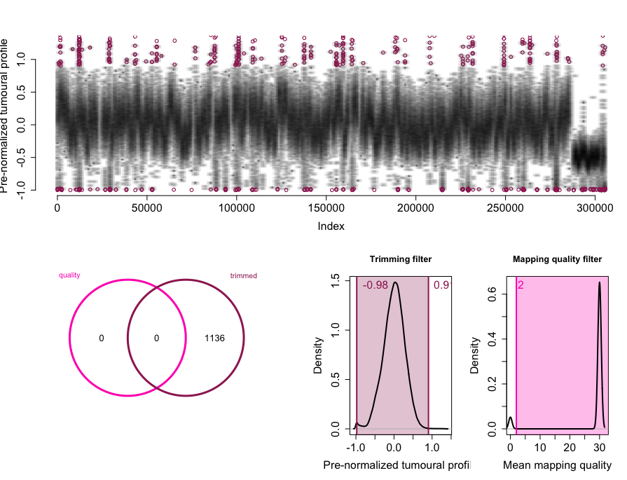
rco = applyFilters(rco, trim.filter=1, mapq.filter=2)
rco = runSeqnorm(rco)
rco = runGLAD(rco)
plotCNProfile(rco)
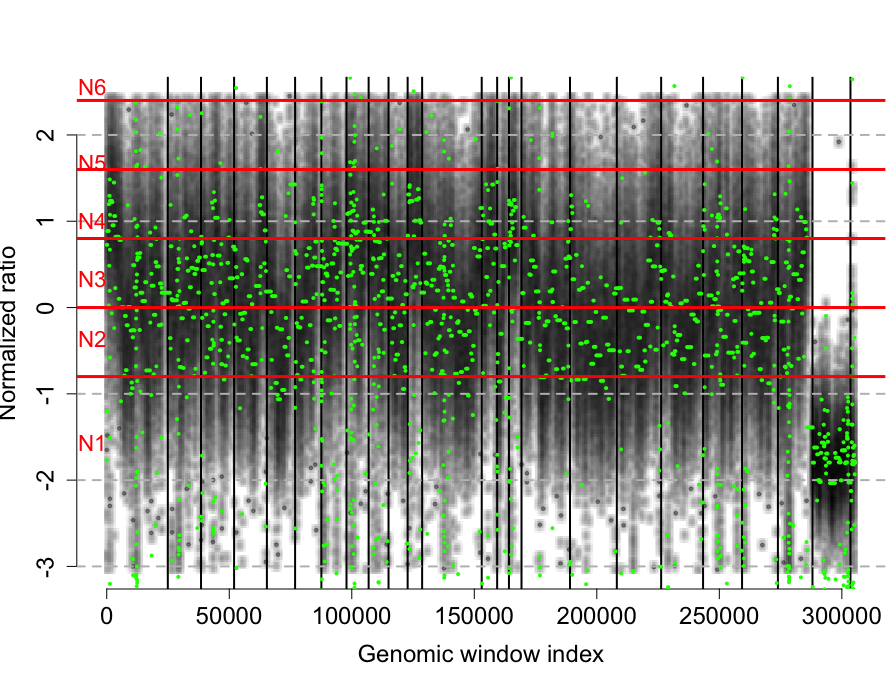
rco = applyThresholds(rco, seq(-0.8,4,by=0.8), 1)
plotCNProfile(rco)
summary(rco)
head(rco@output)
writeCNProfile(rco,'./')虽然其算法比较复杂,但是用法很简单,对input的数据进行了多步骤处理,而且其input数据本身是比较简单的,如下:
> head(seqsumm_HCC1143)
  chrom win.start reads.gc reads.mapq counts
1  chr1     0e+00    0.551      1.691   1199
2  chr1     2e+05    0.534      0.620    824
3  chr1     4e+05    0.457      0.831   8469
4  chr1     6e+05    0.545      6.479   1459
5  chr1     8e+05    0.720     31.619   1094
6  chr1     1e+06    0.766     38.205    976
> dim(seqsumm_HCC1143)
[1] 5314    5
> tail(seqsumm_HCC1143)
     chrom win.start reads.gc reads.mapq counts
5309  chr5 179800000    0.559     35.081   1946
5310  chr5 180000000    0.568     35.668   1970
5311  chr5 180200000    0.545     34.427   1790
5312  chr5 180400000    0.572     34.286   1569
5313  chr5 180600000    0.586     22.844   1591
5314  chr5 180800000    0.562      0.319    845
就是对单个样本的bam文件进行200kb的窗口进行滑动计算每个窗口的gc含量,该窗口区域覆盖的reads数量,还有比对的质量值,很容易写脚本进行计算。
GENOME='/home/jianmingzeng/reference/genome/human_g1k_v37/human_g1k_v37.fasta'
bam='ESCC13-T1_recal.bam'
samtools mpileup -f $GENOME $bam |\
perl -alne '{$pos=int($F[1]/200000); $key="$F[0]\t$pos";$GC{$key}++ if $F[2]=~/[GC]/;$counts_sum{$key}+=$F[3];$number{$key}++;}END{print "$_\t$number{$_}\t$GC{$_}\t$counts_sum{$_}" foreach keys %number}' |\
sort -k1,1 -k 2,2n >T1.windows
得到的结果如下:
head GC_stat.10k.txt
chr1	1	7936	3885	582219
chr1	2	2123	934	88167
chr1	3	1969	169	28729
chr1	4	3556	593	48724
chr1	5	8828	2582	176627
chr1	6	8229	2290	117675
chr1	7	8794	438	156158
chr1	8	10000	723	211816
chr1	9	9077	2421	247285
chr1	10	9415	1661	371830
前面两行是窗口的坐标,第几号染色体的第几个窗口,后面3行是数据,分别是每个窗口的测到的碱基数,GC碱基数,测序总深度。
library(seqCNA)
a=read.table('wgs/GC_stat.10k.txt',fill = T)
a=na.omit(a)
a$GC = a[,4]/a[,3]
a$depth = a[,5]/a[,3]
a = a[a$depth<100,]
plot(a$GC,a$depth)

a=a[,c(1,2,6,5)]
colnames(a)=c('chrom','win.start','reads.gc','counts')
a$counts=floor(a$counts/150)
a$reads.mapq=30
library(seqCNA)
head(a)
dim(a)
tail(a)

a$win.start=a$win.start*10000
a=a[a$chrom %in% paste0('chr',c(1:22,'X','Y')),]
a=a[a$win.start>0,]
a=a[a$counts>0,]
a=a[a$reads.gc>0,]
a=a[,c(1:3,5,4)]

## 200Kb windows to calculate the GC content and counts.
rco = readSeqsumm(tumour.data=a)
rco = applyFilters(rco, trim.filter=1, mapq.filter=2)
rco = runSeqnorm(rco)
rco = runGLAD(rco)
plotCNProfile(rco)
rco = applyThresholds(rco, seq(-0.8,4,by=0.8), 1)
plotCNProfile(rco)
summary(rco)
head(rco@output)
writeCNProfile(rco,'./')Basic information:
SeqCNAInfo object with 306397 10Kbp-long windows.
PEM information is not available.
Paired normal is not available.
Genome and build unknown (chromosomes chr1 to chrY).
Total filtered windows: 23717.
The profile is normalized and segmented.
Copy numbers called from 1 to 8.
CN1:34924 windows.
CN2:95226 windows.
CN3:116829 windows.
CN4:35047 windows.
CN5:554 windows.
CN6:100 windows.
CN7:0 windows.
CN8:0 windows.
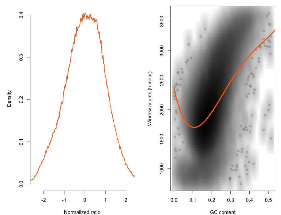
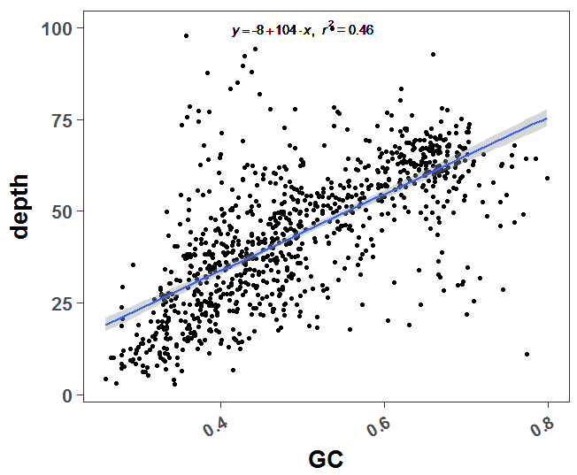
这个是二代测序本身的技术限制,很容易探究到测序深度和GC含量是显著相关的,代码如下:
a=read.table('T1.windows')
a$GC = a[,4]/a[,3]
a$depth = a[,5]/a[,3]
a = a[a$depth<100,]
plot(a$GC,a$depth)
library(ggplot2)
# GET EQUATION AND R-SQUARED AS STRING
# SOURCE: http://goo.gl/K4yh
lm_eqn <- function(x,y){
m <- lm(y ~ x);
eq <- substitute(italic(y) == a + b %.% italic(x)*","~~italic(r)^2~"="~r2,
list(a = format(coef(m)[1], digits = 2),
b = format(coef(m)[2], digits = 2),
r2 = format(summary(m)$r.squared, digits = 3)))
as.character(as.expression(eq));
}
p=ggplot(a,aes(GC,depth)) + geom_point() +
geom_smooth(method='lm',formula=y~x)+
geom_text(x = 0.5, y = 100, label = lm_eqn(a$GC , a$depth), parse = TRUE)
p=p+theme_set(theme_set(theme_bw(base_size=20)))
p=p+theme(text=element_text(face='bold'),
axis.text.x=element_text(angle=30,hjust=1,size =15),
plot.title = element_text(hjust = 0.5) ,
panel.grid = element_blank(),
#panel.border = element_blank()
)
print(p)
可以很明显看到GC含量和测序深度是高度相关的
VarScan v2.2.4 以及更新的版本里面添加了这个分析,主要是针对matched tumor-normal pairs的WES数据来进行分析,得到的是肿瘤测序数据相当于其正常组织测序结果的拷贝数变化情况。输出文件是经典的chromosome, start, stop, and log-base-2 of the copy number change 与拷贝数芯片输出结果类似,所以这个结果可以被bioconductor的DNAcopy包来进行segment算法处理。
详细用法见:http://varscan.sourceforge.net/copy-number-calling.html
这里选取的是前面博文 ESCC-肿瘤空间异质性探究 | 生信菜鸟团 提到的数据,如下:
-r--r--r-- 1 jianmingzeng jianmingzeng 17G Sep 22 00:01 ESCC13-N_recal.bam
-r--r--r-- 1 jianmingzeng jianmingzeng 22G Sep 22 02:09 ESCC13-T1_recal.bam
-r--r--r-- 1 jianmingzeng jianmingzeng 21G Sep 22 01:59 ESCC13-T2_recal.bam
-r--r--r-- 1 jianmingzeng jianmingzeng 16G Sep 21 23:29 ESCC13-T3_recal.bam
-r--r--r-- 1 jianmingzeng jianmingzeng 17G Sep 22 00:32 ESCC13-T4_recal.bam
是同一个病人的4个不同部位的肿瘤,共享同一个正常对照测序数据。
normal='/home/jianmingzeng/data/public/escc/bam/ESCC13-N_recal.bam'
GENOME='/home/jianmingzeng/reference/genome/human_g1k_v37/human_g1k_v37.fasta'
for tumor in /home/jianmingzeng/data/public/escc/bam/*-T*.bam
do
start=$(date +%s.%N)
echo  `date`

file=$(basename $tumor)
sample=${file%%.*}
echo calling $sample

samtools mpileup -q 1 -f $GENOME $normal $tumor |\
awk -F"\t" '$4 > 0 && $7 > 0' |\
java -jar ~/biosoft/VarScan/VarScan.v2.3.9.jar copynumber - $sample --mpileup 1

echo  `date`
dur=$(echo "$(date +%s.%N) - $start" | bc)
printf "Execution time for $sample : %.6f seconds" $dur
echo
done
不过该软件似乎是在这个地方有一个bugs,我也是查了biostar论坛才发现的。主要是两个样本的mpileup文件不能有0,所以需要过滤一下。
这个步骤会产生以copynumber为后缀的输出文件,内容如下:
chrom	chr_start	chr_stop	num_positions	normal_depth	tumor_depth	log2_ratio	gc_content
1	10023	10122	100	14.5	11.1	-0.382	50.0
1	10123	10163	41	15.3	12.4	-0.306	53.7
1	10165	10175	11	12.2	11.5	-0.089	54.5
1	10180	10215	36	11.0	10.9	-0.015	50.0
1	12949	13048	100	17.5	17.0	-0.041	62.0
1	13049	13148	100	26.5	32.9	0.314	61.0
1	13149	13248	100	50.2	52.2	0.056	57.0
1	13249	13348	100	59.7	79.3	0.409	60.0
1	13349	13448	100	56.4	70.1	0.313	53.0
众所周知,以illumina为代表的二代测序对不同GC含量的片段测序效率不同,需要进行校正。而上一个步骤记录了每个片段的GC含量,所以这个步骤就用算法校正一下。
java -jar ~/biosoft/VarScan/VarScan.v2.3.9.jar copyCaller ESCC13-T1_recal.copynumber --output-file varScan.T1.cnv.called似乎挑选标准比较简单,而且出来的结果太多了。
Reading input from ESCC13-T1_recal.copynumber
1959962 raw regions parsed
498738 met min depth
498738 met min size
206188 regions (20520229 bp) were called amplification (log2 > 0.25)
194622 regions (19384202 bp) were called neutral
97928 regions (9726174 bp) were called deletion (log2 <-0.25)
213 regions (20539 bp) were called homozygous deletion (normal cov >= 20 and tumor cov <= 5)
rm(list=ls())
library(DNAcopy)
a=read.table('varScan/varScan.T3.cnv.called',stringsAsFactors = F,header = T)
head(a)
CNA.object <- CNA(cbind( a$adjusted_log_ratio),
                  a$chrom,a$chr_start,
                  data.type="logratio",sampleid="T3")

smoothed.CNA.object <- smooth.CNA(CNA.object)
segment.smoothed.CNA.object <- segment(smoothed.CNA.object, verbose=1)
sdundo.CNA.object <- segment(smoothed.CNA.object,
                             undo.splits="sdundo",
                             undo.SD=3,verbose=1)
head(sdundo.CNA.object$output)
dim(sdundo.CNA.object$output)
dim(sdundo.CNA.object$data)
dim(sdundo.CNA.object$segRows)
head(sdundo.CNA.object$segRows)
tail(sdundo.CNA.object$segRows)
save.image(file = 'DNAcopy_T3.Rdata')近50万行的数据经过了segment算法得到了三千多个拷贝数变异区域,但是有不少区域非常短,其实是需要进一步过滤的。
> head(sdundo.CNA.object$output)
  ID chrom loc.start loc.end num.mark seg.mean
1 T3     1     13049 1666302     1548  -0.2183
2 T3     1   1669546 1684191       11  -0.9250
3 T3     1   1684291 2704373     1037  -0.1705
4 T3     1   2705756 2705956        3  -1.7230
5 T3     1   2706056 6647084     1568  -0.2122
6 T3     1   6647184 6647584        5   0.6866
> dim(sdundo.CNA.object$output)
[1] 3079    6
> dim(sdundo.CNA.object$data)
[1] 499065      3
> dim(sdundo.CNA.object$segRows)
[1] 3079    2
> head(sdundo.CNA.object$segRows)
  startRow endRow
1        1   1548
2     1549   1559
3     1560   2596
4     2597   2599
5     2600   4167
6     4168   4172
> tail(sdundo.CNA.object$segRows)
     startRow endRow
3074   497115 498045
3075   498046 498048
3076   498049 498782
3077   498783 498785
3078   498786 498903
3079   498904 499065
找到拷贝数变异后,除了需要过滤,还需要进行注释,如果有多个样本,还需要在群体里面找寻找recurrent copy number alterations (RCNAs)
比如下面的文章:
We recently published Correlation Matrix Diagonal Segmentation (CMDS) to search for RCNAs using SNP array-based copy number data, and this program can be applied to exome-based copy number data as well.
conifer全称是COpy Number Inference From Exome Reads,发表于2012,目前(2017)已有近300的引用啦。软件本身下载即可使用,但是依赖一下python的包,比如 NumPy and PyTables packages,还有pysam 和matplotlib.
cd ~/biosoft
# http://conifer.sourceforge.net/download.html
mkdir conifer &&  cd conifer
wget https://downloads.sourceforge.net/project/conifer/CoNIFER%200.2.2/conifer_v0.2.2.tar.gz
tar zxvf conifer_v0.2.2.tar.gz
mkdir test && cd test
wget http://sourceforge.net/projects/conifer/files/sampledata.tar.gz
tar zxvf sampledata.tar.gz
wget http://sourceforge.net/projects/conifer/files/probes.txt

python -c "import numpy"
python -c "import tables"
# pip install pysam --user
python -c "import pysam"
python -c "import matplotlib"因为这个软件就是设计给WES测序数据的,所以需要自行制作外显子的坐标记录文件,或者直接下载This file defines the chr:start-stop coordinates for the probes/targets in the exome capture。You can download the standard probe file used in Krumm et al. here. 软件有详细的使用教程:http://conifer.sourceforge.net/tutorial.html
 python conifer.py rpkm \
	--probes probes.txt \
	--input sample.bam \
	--output RPKM/sample.rpkm.txt
**这个程序也是槽点满满,**软件本身只提供了hg19版本的probes.txt文件,反正我各种自己制作都不符合要求,最后得到的每个外显子的RPKM都是几个亿,完全是一脸蒙圈。后来我干脆自己计算RPKM啦,代码如下:
bed=exon_probe.hg38.gene.bed
for bam in  *bam
do
file=$(basename $bam )
sample=${file%%.*}
echo $sample
#export total_reads=$(samtools view -F 0x4 $bam | cut -f 1 | sort | uniq | wc -l)
export total_reads=$(samtools idxstats  $bam|awk -F '\t' '{s+=$3}END{print s}')
echo The number of reads is $total_reads
bedtools multicov -bams  $bam -bed $bed |perl -alne '{$len=$F[2]-$F[1];if($len <1 ){print "$.\t$F[4]\t0" }else{$rpkm=(1000000000*$F[4]/($len* $ENV{total_reads}));print "$.\t$F[4]\t$rpkm"}}' >$sample.rpkm.txt
done
上面那个exon_probe.hg38.gene.bed文件我是下载了CCDS文件制作的。
wget ftp://ftp.ncbi.nlm.nih.gov/pub/CCDS/current_human/CCDS.20160908.txt
cat CCDS.20160908.txt |perl -alne '{/\[(.*?)\]/;next unless $1;$gene=$F[2];$exons=$1;$exons=~s/\s//g;$exons=~s/-/\t/g;print "$F[0]\t$_\t$gene" foreach split/,/,$exons;}'|sort -u |bedtools sort -i > exon_probe.grch38.gene.bed
sed 's/^/chr/g' exon_probe.grch38.gene.bed >exon_probe.hg38.gene.bed
不过作者给了测试就,是The sample data set of 26 RPKM files. Sample RPKM Files
| Study | Exome Capture | N | Samples |
|---|---|---|---|
| HapMap | Nimblegen V1 (2009) | 8 | NA12878, NA15510, NA18507, NA18517, NA18555, NA18956, NA19129, NA19240 |
| Autism Trios | Nimblegen V2 (2010) | 18 | 6 Trios (Mother, Father, Proband) |
这里就用这个测试数据来说明这个软件的用法吧,很明显,需要多个样本一起运行。
中间报错了,日志如下:
File "conifer.py", line 682, in <module>
args.func(args)
File "conifer.py", line 564, in CF_bam2RPKM
if not f._hasIndex():
简单谷歌了一下,发现了解决方案,需要修改那个conifer.py 程序,这么大一个bug作者居然不去修复,真奇怪。解决方案如下:
It's a very simple fix. Just change line 564 of conifer.py from:
if not f._hasIndex():
to
if not f.has_index():
Then it should work.
代码不复杂,就是WES的探针文件,加上转换好的RPKM文件即可。
 cd ~/biosoft/conifer/test/
 python ~/biosoft/conifer/conifer_v0.2.2/conifer.py analyze \
  	--probes ~/biosoft/conifer/test/probes.txt \
  	--rpkm_dir ~/biosoft/conifer/test/sampledata/RPKM_data/  \
  	--output analysis.hdf5 \
  	--svd 6 \
  	--write_svals singular_values.txt \
  	--plot_scree screeplot.png \
--write_sd sd_values.txt cd ~/biosoft/conifer/test/
python ~/biosoft/conifer/conifer_v0.2.2/conifer.py call \
--input analysis.hdf5 \
--output calls.txt这里得到的calls.txt就是我们对这个WES项目的CNV分析结果啦
$ head calls.txt
sampleID	chromosome	start	stop	state
Trio2.fa	chr1	196714946	196759357	del
NA18555	chr1	161483684	161640062	dup
NA15510	chr1	155226464	155261728	dup
Trio3.mo	chr1	149398798	149760173	del
NA19240	chr1	110224430	110254970	dup
Trio3.fa	chr10	46998880	47894049	dup
Trio3.fa	chr10	47948713	48382260	dup
Trio4.fa	chr10	124362280	124370763	dup
NA18956 chr10 124342115 124352111 del cd ~/biosoft/conifer/test/
mkdir export_svdzrpkm/
python ~/biosoft/conifer/conifer_v0.2.2/conifer.py export \
--input analysis.hdf5 \
--output ./export_svdzrpkm/
## 需要自定义区域进行可视化
cd ~/biosoft/conifer/test/
python ~/biosoft/conifer/conifer_v0.2.2/conifer.py plot \
--input analysis.hdf5 \
--region chr#:start-stop \
--output image.png \
--sample sampleID
## 也可以一次性画出所有的图
cd ~/biosoft/conifer/test/
mkdir call_imgs/
python ~/biosoft/conifer/conifer_v0.2.2/conifer.py plotcalls \
--input analysis.hdf5
--calls calls.txt
--outputdir ./call_imgs/
Legend/Explanation: X-axis: Exons/probes from the probes.txt file Y-axis: SVD-ZRPKM values for each exon. Red bars and line: SVD-ZRPKM values for each exon from the sample with the call (or highlighted sample). The smooth continuous line is simply a gaussian-smoothed representation of the SVD-ZRPKM values at each exon. Thin black in background: All other samples in the analysis (for comparison and simultaneous visualization purposes) Purple bars: Genes from the probes.txt file Black bar: If using the "plotcalls" command, this bar will indicate extent of call above threshold (--threshold) value.
目前主流检测全基因组水平拷贝数变异(CNV)的平台主要是基因芯片,但是基因芯片一般来说检测的片段长度至少在10kb以上,另外对于特定区域的拷贝数,如DMD等,还可以使用MLPA平台,对于全外显子来说,其本身设计是用来检测点突变与indel的,由于实验与基因数据分析技术的局限,全外显子CNV分析有很高的假阳性,所以常规流程中并不包括全外显子CNV分析,可是在实际的科研与临床工作中,在排除了点突变与indel之后仍然找不到有意义的变异之后,分析CNV成为最后的希望。
基因检测与解读公众号的游侠推荐过相对比较靠谱的两款分析软件:XHMM与CODEX。
-
XHMM(exome hidden Markov model)软件由美国纽约西奈山医学院的Fromer等开发,发表于2012年10月的Am J Hum Genet杂志(PMID:23040492),XHMM的主要原理是:通过GATK的Depth of Coverage工具计算每个外显子的测序深度,然后PCA将不同样本的深度进行归一化,去除高变异的背景噪声,HMM算法训练数据分析哪些属于高深度区域,哪些属于低深度区域,最后拷贝数分析并得出基因型。
-
CODEX软件由宾夕法尼亚大学的Jiang Y等开发,发表于2015年3月的Nucleic Acids Res(PMID: 25618849). CODEX的主要原理是:计算每个外显子的测序深度、比对率及GC含量,归一化每个样本的测序深度,Poisson片段化分析,最后计算每个样本的CNV。
因为暂时用不到,就不写教程了,反正学个软件,就是看readme罢了,想要用的好,就得把readme仔细读下去,并且看发表的文章。
我应该会更新一个CNVkit的使用说明。