The Keras functional API is the way to go for defining complex models, such as multi-output models, directed acyclic graphs, or models with shared layers.

First example: a densely-connected network

The Sequential model is probably a better choice to implement such a network, but it helps to start with something really simple.

-> A layer instance is callable (on a tensor), and it returns a tensor -> Input tensor(s) and output tensor(s) can then be used to define a Model -> Such a model can be trained just like Keras Sequential models.

from keras.layers import Input, Dense
from keras.models import Model

# This returns a tensor
inputs = Input(shape=(784,))

# a layer instance is callable on a tensor, and returns a tensor
x = Dense(64, activation='relu')(inputs)
x = Dense(64, activation='relu')(x)
predictions = Dense(10, activation='softmax')(x)

# This creates a model that includes
# the Input layer and three Dense layers
model = Model(inputs=inputs, outputs=predictions)
model.compile(optimizer='rmsprop',
              loss='categorical_crossentropy',
              metrics=['accuracy'])
model.fit(data, labels)  # starts training

All models are callable, just like layers With the functional API, it is easy to reuse trained models: you can treat any model as if it were a layer, by calling it on a tensor. Note that by calling a model you aren't just reusing the architecture of the model, you are also reusing its weights.

x = Input(shape=(784,))
# This works, and returns the 10-way softmax we defined above.
y = model(x)

Here's a good use case for the functional API: models with multiple inputs and outputs. The functional API makes it easy to manipulate a large number of intertwined datastreams.

Let's consider the following model. We seek to predict how many retweets and likes a news headline will receive on Twitter. The main input to the model will be the headline itself, as a sequence of words, but to spice things up, our model will also have an auxiliary input, receiving extra data such as the time of day when the headline was posted, etc. The model will also be supervised via two loss functions. Using the main loss function earlier in a model is a good regularization mechanism for deep models.

Here's what our model looks like:

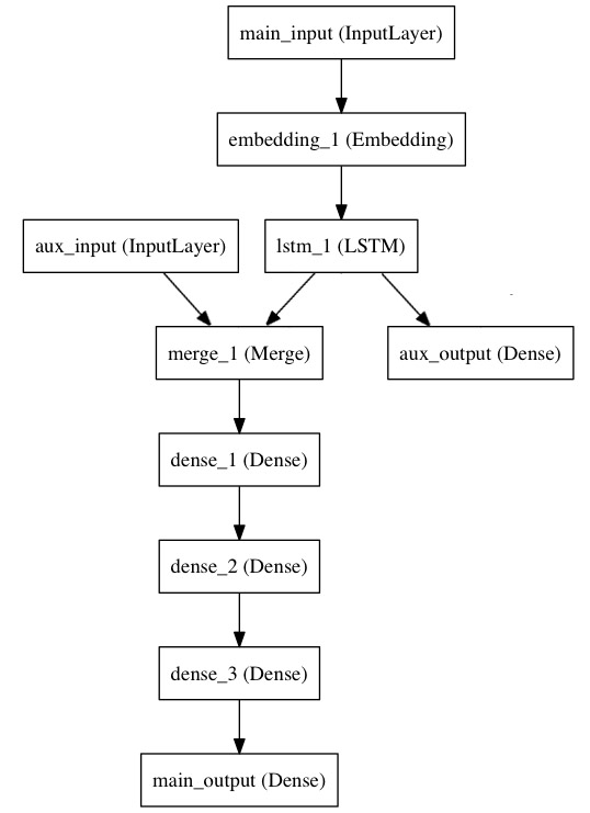
Let's implement it with the functional API.

The main input will receive the headline, as a sequence of integers (each integer encodes a word). The integers will be between 1 and 10,000 (a vocabulary of 10,000 words) and the sequences will be 100 words long.

from keras.layers import Input, Embedding, LSTM, Dense
from keras.models import Model

# Headline input: meant to receive sequences of 100 integers, between 1 and 10000.
# Note that we can name any layer by passing it a "name" argument.
main_input = Input(shape=(100,), dtype='int32', name='main_input')

# This embedding layer will encode the input sequence
# into a sequence of dense 512-dimensional vectors.
x = Embedding(output_dim=512, input_dim=10000, input_length=100)(main_input)

# A LSTM will transform the vector sequence into a single vector,
# containing information about the entire sequence
lstm_out = LSTM(32)(x)

Here we insert the auxiliary loss, allowing the LSTM and Embedding layer to be trained smoothly even though the main loss will be much higher in the model.

auxiliary_output = Dense(1, activation='sigmoid', name='aux_output')(lstm_out)

At this point, we feed into the model our auxiliary input data by concatenating it with the LSTM output:

auxiliary_input = Input(shape=(5,), name='aux_input')
x = keras.layers.concatenate([lstm_out, auxiliary_input])

# We stack a deep densely-connected network on top
x = Dense(64, activation='relu')(x)
x = Dense(64, activation='relu')(x)
x = Dense(64, activation='relu')(x)

# And finally we add the main logistic regression layer
main_output = Dense(1, activation='sigmoid', name='main_output')(x)

This defines a model with two inputs and two outputs:

model = Model(inputs=[main_input, auxiliary_input], outputs=[main_output, auxiliary_output])

We compile the model and assign a weight of 0.2 to the auxiliary loss. To specify different loss_weights or loss for each different output, you can use a list or a dictionary. Here we pass a single loss as the loss argument, so the same loss will be used on all outputs.

model.compile(optimizer='rmsprop', loss='binary_crossentropy', loss_weights=[1., 0.2])

We can train the model by passing it lists of input arrays and target arrays:

model.fit([headline_data, additional_data], [labels, labels], epochs=50, batch_size=32)

Since our inputs and outputs are named (we passed them a "name" argument), we could also have compiled the model via:

model.compile(optimizer='rmsprop',
              loss={'main_output': 'binary_crossentropy', 'aux_output': 'binary_crossentropy'},
              loss_weights={'main_output': 1., 'aux_output': 0.2})

# And trained it via:
model.fit({'main_input': headline_data, 'aux_input': additional_data},
          {'main_output': labels, 'aux_output': labels},
          epochs=50, batch_size=32)

Another good use for the functional API are models that use shared layers. Let's take a look at shared layers.

Let's consider a dataset of tweets. We want to build a model that can tell whether two tweets are from the same person or not (this can allow us to compare users by the similarity of their tweets, for instance).

One way to achieve this is to build a model that encodes two tweets into two vectors, concatenates the vectors and then adds a logistic regression; this outputs a probability that the two tweets share the same author. The model would then be trained on positive tweet pairs and negative tweet pairs.

Because the problem is symmetric, the mechanism that encodes the first tweet should be reused (weights and all) to encode the second tweet. Here we use a shared LSTM layer to encode the tweets.

Let's build this with the functional API. We will take as input for a tweet a binary matrix of shape (280, 256), i.e. a sequence of 280 vectors of size 256, where each dimension in the 256-dimensional vector encodes the presence/absence of a character (out of an alphabet of 256 frequent characters).

import keras
from keras.layers import Input, LSTM, Dense
from keras.models import Model

tweet_a = Input(shape=(280, 256))
tweet_b = Input(shape=(280, 256))

To share a layer across different inputs, simply instantiate the layer once, then call it on as many inputs as you want:

# This layer can take as input a matrix
# and will return a vector of size 64
shared_lstm = LSTM(64)

# When we reuse the same layer instance
# multiple times, the weights of the layer
# are also being reused
# (it is effectively *the same* layer)
encoded_a = shared_lstm(tweet_a)
encoded_b = shared_lstm(tweet_b)

# We can then concatenate the two vectors:
merged_vector = keras.layers.concatenate([encoded_a, encoded_b], axis=-1)

# And add a logistic regression on top
predictions = Dense(1, activation='sigmoid')(merged_vector)

# We define a trainable model linking the
# tweet inputs to the predictions
model = Model(inputs=[tweet_a, tweet_b], outputs=predictions)

model.compile(optimizer='rmsprop',
              loss='binary_crossentropy',
              metrics=['accuracy'])
model.fit([data_a, data_b], labels, epochs=10)

Let's pause to take a look at how to read the shared layer's output or output shape.

Whenever you are calling a layer on some input, you are creating a new tensor (the output of the layer), and you are adding a "node" to the layer, linking the input tensor to the output tensor. When you are calling the same layer multiple times, that layer owns multiple nodes indexed as 0, 1, 2...

In previous versions of Keras, you could obtain the output tensor of a layer instance via layer.get_output(), or its output shape via layer.output_shape. You still can (except get_output() has been replaced by the property output). But what if a layer is connected to multiple inputs?

As long as a layer is only connected to one input, there is no confusion, and .output will return the one output of the layer:

a = Input(shape=(280, 256))

lstm = LSTM(32)
encoded_a = lstm(a)

assert lstm.output == encoded_a

Not so if the layer has multiple inputs:

a = Input(shape=(280, 256))
b = Input(shape=(280, 256))

lstm = LSTM(32)
encoded_a = lstm(a)
encoded_b = lstm(b)

lstm.output
>> AttributeError: Layer lstm_1 has multiple inbound nodes,
hence the notion of "layer output" is ill-defined.
Use `get_output_at(node_index)` instead.

Okay then. The following works:

assert lstm.get_output_at(0) == encoded_a
assert lstm.get_output_at(1) == encoded_b

Simple enough, right?

The same is true for the properties input_shape and output_shape: as long as the layer has only one node, or as long as all nodes have the same input/output shape, then the notion of "layer output/input shape" is well defined, and that one shape will be returned by layer.output_shape/layer.input_shape. But if, for instance, you apply the same Conv2D layer to an input of shape (32, 32, 3), and then to an input of shape (64, 64, 3), the layer will have multiple input/output shapes, and you will have to fetch them by specifying the index of the node they belong to:

a = Input(shape=(32, 32, 3))
b = Input(shape=(64, 64, 3))

conv = Conv2D(16, (3, 3), padding='same')
conved_a = conv(a)

# Only one input so far, the following will work:
assert conv.input_shape == (None, 32, 32, 3)

conved_b = conv(b)
# now the `.input_shape` property wouldn't work, but this does:
assert conv.get_input_shape_at(0) == (None, 32, 32, 3)
assert conv.get_input_shape_at(1) == (None, 64, 64, 3)

Let us go through an example:

Visual question answering model This model can select the correct one-word answer when asked a natural-language question about a picture.

It works by encoding the question into a vector, encoding the image into a vector, concatenating the two, and training on top a logistic regression over some vocabulary of potential answers.

from keras.layers import Conv2D, MaxPooling2D, Flatten
from keras.layers import Input, LSTM, Embedding, Dense
from keras.models import Model, Sequential

# First, let's define a vision model using a Sequential model.
# This model will encode an image into a vector.
vision_model = Sequential()
vision_model.add(Conv2D(64, (3, 3), activation='relu', padding='same', input_shape=(224, 224, 3)))
vision_model.add(Conv2D(64, (3, 3), activation='relu'))
vision_model.add(MaxPooling2D((2, 2)))
vision_model.add(Conv2D(128, (3, 3), activation='relu', padding='same'))
vision_model.add(Conv2D(128, (3, 3), activation='relu'))
vision_model.add(MaxPooling2D((2, 2)))
vision_model.add(Conv2D(256, (3, 3), activation='relu', padding='same'))
vision_model.add(Conv2D(256, (3, 3), activation='relu'))
vision_model.add(Conv2D(256, (3, 3), activation='relu'))
vision_model.add(MaxPooling2D((2, 2)))
vision_model.add(Flatten())

# Now let's get a tensor with the output of our vision model:
image_input = Input(shape=(224, 224, 3))
encoded_image = vision_model(image_input)

# Next, let's define a language model to encode the question into a vector.
# Each question will be at most 100 word long,
# and we will index words as integers from 1 to 9999.
question_input = Input(shape=(100,), dtype='int32')
embedded_question = Embedding(input_dim=10000, output_dim=256, input_length=100)(question_input)
encoded_question = LSTM(256)(embedded_question)

# Let's concatenate the question vector and the image vector:
merged = keras.layers.concatenate([encoded_question, encoded_image])

# And let's train a logistic regression over 1000 words on top:
output = Dense(1000, activation='softmax')(merged)

# This is our final model:
vqa_model = Model(inputs=[image_input, question_input], outputs=output)

# The next stage would be training this model on actual data.

Unlike the Sequential model, you must create and define a standalone Input layer that specifies the shape of input data.

The input layer takes a shape argument that is a tuple that indicates the dimensionality of the input data.

When input data is one-dimensional, such as for a multilayer Perceptron, the shape must explicitly leave room for the shape of the mini-batch size used when splitting the data when training the network. Therefore, the shape tuple is always defined with a hanging last dimension when the input is one-dimensional (2,), for example:

from keras.layers import Input
visible = Input(shape=(2,))

The layers in the model are connected pairwise.

This is done by specifying where the input comes from when defining each new layer. A bracket notation is used, such that after the layer is created, the layer from which the input to the current layer comes from is specified.

Let’s make this clear with a short example. We can create the input layer as above, then create a hidden layer as a Dense that receives input only from the input layer.

from keras.layers import Input
from keras.layers import Dense
visible = Input(shape=(2,))
hidden = Dense(2)(visible)

Note the (visible) after the creation of the Dense layer that connects the input layer output as the input to the dense hidden layer.

It is this way of connecting layers piece by piece that gives the functional API its flexibility. For example, you can see how easy it would be to start defining ad hoc graphs of layers.

After creating all of your model layers and connecting them together, you must define the model.

As with the Sequential API, the model is the thing you can summarize, fit, evaluate, and use to make predictions.

Keras provides a Model class that you can use to create a model from your created layers. It requires that you only specify the input and output layers. For example:

from keras.models import Model
from keras.layers import Input
from keras.layers import Dense
visible = Input(shape=(2,))
hidden = Dense(2)(visible)
model = Model(inputs=visible, outputs=hidden)

Now that we know all of the key pieces of the Keras functional API, let’s work through defining a suite of different models and build up some practice with it.

Each example is executable and prints the structure and creates a diagram of the graph. I recommend doing this for your own models to make it clear what exactly you have defined.

My hope is that these examples provide templates for you when you want to define your own models using the functional API in the future.

When getting started with the functional API, it is a good idea to see how some standard neural network models are defined.

In this section, we will look at defining a simple multilayer Perceptron, convolutional neural network, and recurrent neural network.

These examples will provide a foundation for understanding the more elaborate examples later.

Multilayer Perceptron In this section, we define a multilayer Perceptron model for binary classification.

The model has 10 inputs, 3 hidden layers with 10, 20, and 10 neurons, and an output layer with 1 output. Rectified linear activation functions are used in each hidden layer and a sigmoid activation function is used in the output layer, for binary classification.

# Multilayer Perceptron
from keras.utils import plot_model
from keras.models import Model
from keras.layers import Input
from keras.layers import Dense
visible = Input(shape=(10,))
hidden1 = Dense(10, activation='relu')(visible)
hidden2 = Dense(20, activation='relu')(hidden1)
hidden3 = Dense(10, activation='relu')(hidden2)
output = Dense(1, activation='sigmoid')(hidden3)
model = Model(inputs=visible, outputs=output)
# summarize layers
print(model.summary())
# plot graph
plot_model(model, to_file='multilayer_perceptron_graph.png')

Running the example prints the structure of the network.

input_1 (InputLayer) (None, 10) 0

dense_1 (Dense) (None, 10) 110

dense_2 (Dense) (None, 20) 220

dense_3 (Dense) (None, 10) 210

Total params: 551 Trainable params: 551 Non-trainable params: 0

A plot of the model graph is also created and saved to file.

Convolutional Neural Network In this section, we will define a convolutional neural network for image classification.

The model receives black and white 64×64 images as input, then has a sequence of two convolutional and pooling layers as feature extractors, followed by a fully connected layer to interpret the features and an output layer with a sigmoid activation for two-class predictions.

# Convolutional Neural Network
from keras.utils import plot_model
from keras.models import Model
from keras.layers import Input
from keras.layers import Dense
from keras.layers import Flatten
from keras.layers.convolutional import Conv2D
from keras.layers.pooling import MaxPooling2D
visible = Input(shape=(64,64,1))
conv1 = Conv2D(32, kernel_size=4, activation='relu')(visible)
pool1 = MaxPooling2D(pool_size=(2, 2))(conv1)
conv2 = Conv2D(16, kernel_size=4, activation='relu')(pool1)
pool2 = MaxPooling2D(pool_size=(2, 2))(conv2)
flat = Flatten()(pool2)
hidden1 = Dense(10, activation='relu')(flat)
output = Dense(1, activation='sigmoid')(hidden1)
model = Model(inputs=visible, outputs=output)
# summarize layers
print(model.summary())
# plot graph
plot_model(model, to_file='convolutional_neural_network.png')
Running the example summarizes the model layers.

input_1 (InputLayer) (None, 64, 64, 1) 0

conv2d_1 (Conv2D) (None, 61, 61, 32) 544

max_pooling2d_1 (MaxPooling2 (None, 30, 30, 32) 0

conv2d_2 (Conv2D) (None, 27, 27, 16) 8208

max_pooling2d_2 (MaxPooling2 (None, 13, 13, 16) 0

flatten_1 (Flatten) (None, 2704) 0

dense_1 (Dense) (None, 10) 27050

Total params: 35,813 Trainable params: 35,813 Non-trainable params: 0

A plot of the model graph is also created and saved to file.

In this section, we will define a long short-term memory recurrent neural network for sequence classification.

The model expects 100 time steps of one feature as input. The model has a single LSTM hidden layer to extract features from the sequence, followed by a fully connected layer to interpret the LSTM output, followed by an output layer for making binary predictions.

# Recurrent Neural Network
from keras.utils import plot_model
from keras.models import Model
from keras.layers import Input
from keras.layers import Dense
from keras.layers.recurrent import LSTM
visible = Input(shape=(100,1))
hidden1 = LSTM(10)(visible)
hidden2 = Dense(10, activation='relu')(hidden1)
output = Dense(1, activation='sigmoid')(hidden2)
model = Model(inputs=visible, outputs=output)
# summarize layers
print(model.summary())
# plot graph
plot_model(model, to_file='recurrent_neural_network.png')

Running the example summarizes the model layers.

input_1 (InputLayer) (None, 100, 1) 0

lstm_1 (LSTM) (None, 10) 480

dense_1 (Dense) (None, 10) 110

Total params: 601 Trainable params: 601 Non-trainable params: 0

A plot of the model graph is also created and saved to file.

Multiple layers can share the output from one layer.

For example, there may be multiple different feature extraction layers from an input, or multiple layers used to interpret the output from a feature extraction layer.

Let’s look at both of these examples.

Shared Input Layer In this section, we define multiple convolutional layers with differently sized kernels to interpret an image input.

The model takes black and white images with the size 64×64 pixels. There are two CNN feature extraction submodels that share this input; the first has a kernel size of 4 and the second a kernel size of 8. The outputs from these feature extraction submodels are flattened into vectors and concatenated into one long vector and passed on to a fully connected layer for interpretation before a final output layer makes a binary classification.

from keras.utils import plot_model
from keras.models import Model
from keras.layers import Input
from keras.layers import Dense
from keras.layers import Flatten
from keras.layers.convolutional import Conv2D
from keras.layers.pooling import MaxPooling2D
from keras.layers.merge import concatenate
# input layer
visible = Input(shape=(64,64,1))
# first feature extractor
conv1 = Conv2D(32, kernel_size=4, activation='relu')(visible)
pool1 = MaxPooling2D(pool_size=(2, 2))(conv1)
flat1 = Flatten()(pool1)
# second feature extractor
conv2 = Conv2D(16, kernel_size=8, activation='relu')(visible)
pool2 = MaxPooling2D(pool_size=(2, 2))(conv2)
flat2 = Flatten()(pool2)
# merge feature extractors
merge = concatenate([flat1, flat2])
# interpretation layer
hidden1 = Dense(10, activation='relu')(merge)
# prediction output
output = Dense(1, activation='sigmoid')(hidden1)
model = Model(inputs=visible, outputs=output)
# summarize layers
print(model.summary())
# plot graph
plot_model(model, to_file='shared_input_layer.png')

Running the example summarizes the model layers.

input_1 (InputLayer) (None, 64, 64, 1) 0

conv2d_1 (Conv2D) (None, 61, 61, 32) 544 input_1[0][0]

conv2d_2 (Conv2D) (None, 57, 57, 16) 1040 input_1[0][0]

max_pooling2d_1 (MaxPooling2D) (None, 30, 30, 32) 0 conv2d_1[0][0]

max_pooling2d_2 (MaxPooling2D) (None, 28, 28, 16) 0 conv2d_2[0][0]

flatten_1 (Flatten) (None, 28800) 0 max_pooling2d_1[0][0]

flatten_2 (Flatten) (None, 12544) 0 max_pooling2d_2[0][0]

concatenate_1 (Concatenate) (None, 41344) 0 flatten_1[0][0] flatten_2[0][0]

dense_1 (Dense) (None, 10) 413450 concatenate_1[0][0]

Total params: 415,045 Trainable params: 415,045 Non-trainable params: 0

A plot of the model graph is also created and saved to file.

In this section, we will use two parallel submodels to interpret the output of an LSTM feature extractor for sequence classification.

The input to the model is 100 time steps of 1 feature. An LSTM layer with 10 memory cells interprets this sequence. The first interpretation model is a shallow single fully connected layer, the second is a deep 3 layer model. The output of both interpretation models are concatenated into one long vector that is passed to the output layer used to make a binary prediction.

# Shared Feature Extraction Layer
from keras.utils import plot_model
from keras.models import Model
from keras.layers import Input
from keras.layers import Dense
from keras.layers.recurrent import LSTM
from keras.layers.merge import concatenate
# define input
visible = Input(shape=(100,1))
# feature extraction
extract1 = LSTM(10)(visible)
# first interpretation model
interp1 = Dense(10, activation='relu')(extract1)
# second interpretation model
interp11 = Dense(10, activation='relu')(extract1)
interp12 = Dense(20, activation='relu')(interp11)
interp13 = Dense(10, activation='relu')(interp12)
# merge interpretation
merge = concatenate([interp1, interp13])
# output
output = Dense(1, activation='sigmoid')(merge)
model = Model(inputs=visible, outputs=output)
# summarize layers
print(model.summary())
# plot graph
plot_model(model, to_file='shared_feature_extractor.png')

Running the example summarizes the model layers.

input_1 (InputLayer) (None, 100, 1) 0

lstm_1 (LSTM) (None, 10) 480 input_1[0][0]

dense_2 (Dense) (None, 10) 110 lstm_1[0][0]

dense_3 (Dense) (None, 20) 220 dense_2[0][0]

dense_1 (Dense) (None, 10) 110 lstm_1[0][0]

dense_4 (Dense) (None, 10) 210 dense_3[0][0]

concatenate_1 (Concatenate) (None, 20) 0 dense_1[0][0] dense_4[0][0]

Total params: 1,151 Trainable params: 1,151 Non-trainable params: 0

A plot of the model graph is also created and saved to file.

The functional API can also be used to develop more complex models with multiple inputs, possibly with different modalities. It can also be used to develop models that produce multiple outputs.

We will look at examples of each in this section.

Multiple Input Model We will develop an image classification model that takes two versions of the image as input, each of a different size. Specifically a black and white 64×64 version and a color 32×32 version. Separate feature extraction CNN models operate on each, then the results from both models are concatenated for interpretation and ultimate prediction.

Note that in the creation of the Model() instance, that we define the two input layers as an array. Specifically:

model = Model(inputs=[visible1, visible2], outputs=output)

The complete example is listed below.

# Multiple Inputs
from keras.utils import plot_model
from keras.models import Model
from keras.layers import Input
from keras.layers import Dense
from keras.layers import Flatten
from keras.layers.convolutional import Conv2D
from keras.layers.pooling import MaxPooling2D
from keras.layers.merge import concatenate
# first input model
visible1 = Input(shape=(64,64,1))
conv11 = Conv2D(32, kernel_size=4, activation='relu')(visible1)
pool11 = MaxPooling2D(pool_size=(2, 2))(conv11)
conv12 = Conv2D(16, kernel_size=4, activation='relu')(pool11)
pool12 = MaxPooling2D(pool_size=(2, 2))(conv12)
flat1 = Flatten()(pool12)
# second input model
visible2 = Input(shape=(32,32,3))
conv21 = Conv2D(32, kernel_size=4, activation='relu')(visible2)
pool21 = MaxPooling2D(pool_size=(2, 2))(conv21)
conv22 = Conv2D(16, kernel_size=4, activation='relu')(pool21)
pool22 = MaxPooling2D(pool_size=(2, 2))(conv22)
flat2 = Flatten()(pool22)
# merge input models
merge = concatenate([flat1, flat2])
# interpretation model
hidden1 = Dense(10, activation='relu')(merge)
hidden2 = Dense(10, activation='relu')(hidden1)
output = Dense(1, activation='sigmoid')(hidden2)
model = Model(inputs=[visible1, visible2], outputs=output)
# summarize layers
print(model.summary())
# plot graph
plot_model(model, to_file='multiple_inputs.png')

Running the example summarizes the model layers.

input_1 (InputLayer) (None, 64, 64, 1) 0

input_2 (InputLayer) (None, 32, 32, 3) 0

conv2d_1 (Conv2D) (None, 61, 61, 32) 544 input_1[0][0]

conv2d_3 (Conv2D) (None, 29, 29, 32) 1568 input_2[0][0]

max_pooling2d_1 (MaxPooling2D) (None, 30, 30, 32) 0 conv2d_1[0][0]

max_pooling2d_3 (MaxPooling2D) (None, 14, 14, 32) 0 conv2d_3[0][0]

conv2d_2 (Conv2D) (None, 27, 27, 16) 8208 max_pooling2d_1[0][0]

conv2d_4 (Conv2D) (None, 11, 11, 16) 8208 max_pooling2d_3[0][0]

max_pooling2d_2 (MaxPooling2D) (None, 13, 13, 16) 0 conv2d_2[0][0]

max_pooling2d_4 (MaxPooling2D) (None, 5, 5, 16) 0 conv2d_4[0][0]

flatten_1 (Flatten) (None, 2704) 0 max_pooling2d_2[0][0]

flatten_2 (Flatten) (None, 400) 0 max_pooling2d_4[0][0]

concatenate_1 (Concatenate) (None, 3104) 0 flatten_1[0][0] flatten_2[0][0]

dense_1 (Dense) (None, 10) 31050 concatenate_1[0][0]

dense_2 (Dense) (None, 10) 110 dense_1[0][0]

Total params: 49,699 Trainable params: 49,699 Non-trainable params: 0

A plot of the model graph is also created and saved to file.

In this section, we will develop a model that makes two different types of predictions. Given an input sequence of 100 time steps of one feature, the model will both classify the sequence and output a new sequence with the same length.

An LSTM layer interprets the input sequence and returns the hidden state for each time step. The first output model creates a stacked LSTM, interprets the features, and makes a binary prediction. The second output model uses the same output layer to make a real-valued prediction for each input time step.

# Multiple Outputs
from keras.utils import plot_model
from keras.models import Model
from keras.layers import Input
from keras.layers import Dense
from keras.layers.recurrent import LSTM
from keras.layers.wrappers import TimeDistributed
# input layer
visible = Input(shape=(100,1))
# feature extraction
extract = LSTM(10, return_sequences=True)(visible)
# classification output
class11 = LSTM(10)(extract)
class12 = Dense(10, activation='relu')(class11)
output1 = Dense(1, activation='sigmoid')(class12)
# sequence output
output2 = TimeDistributed(Dense(1, activation='linear'))(extract)
# output
model = Model(inputs=visible, outputs=[output1, output2])
# summarize layers
print(model.summary())
# plot graph
plot_model(model, to_file='multiple_outputs.png')

Running the example summarizes the model layers.

input_1 (InputLayer) (None, 100, 1) 0

lstm_1 (LSTM) (None, 100, 10) 480 input_1[0][0]

lstm_2 (LSTM) (None, 10) 840 lstm_1[0][0]

dense_1 (Dense) (None, 10) 110 lstm_2[0][0]

dense_2 (Dense) (None, 1) 11 dense_1[0][0]

Total params: 1,452 Trainable params: 1,452 Non-trainable params: 0

A plot of the model graph is also created and saved to file.

In this section, I want to give you some tips to get the most out of the functional API when you are defining your own models.

Consistent Variable Names. Use the same variable name for the input (visible) and output layers (output) and perhaps even the hidden layers (hidden1, hidden2). It will help to connect things together correctly. Review Layer Summary. Always print the model summary and review the layer outputs to ensure that the model was connected together as you expected. Review Graph Plots. Always create a plot of the model graph and review it to ensure that everything was put together as you intended. Name the layers. You can assign names to layers that are used when reviewing summaries and plots of the model graph. For example: Dense(1, name=’hidden1′). Separate Submodels. Consider separating out the development of submodels and combine the submodels together at the end.

If you are new or new-ish to Python the syntax used in the functional API may be confusing.

For example, given:

...
dense1 = Dense(32)(input)
...

What does the double bracket syntax do?

What does it mean?

It looks confusing, but it is not a special python thing, just one line doing two things.

The first bracket “(32)” creates the layer via the class constructor, the second bracket “(input)” is a function with no name implemented via the call() function, that when called will connect the layers.

The call() function is a default function on all Python objects that can be overridden and is used to “call” an instantiated object. Just like the init() function is a default function on all objects called just after instantiating an object to initialize it.

We can do the same thing in two lines:

# create layer
dense1 = Dense(32)
# connect layer to previous layer
dense1(input)

I guess we could also call the call() function on the object explicitly, although I have never tried:

# create layer
dense1 = Dense(32)
# connect layer to previous layer
dense1.__call_(input)