Welcome to NETPolynomial! This library is written to provide single and multivariate polynomial representation for .NET framework users. Additionally, it allows its users to evaluate polynomial values, provided that coefficients and indeterminates are defined.

NETPolynomial offers a mechanism of representing and evaluating polynomials using .NET framework. Supported are polynomials consisting of finite number of terms, indeterminates, coefficients and of degrees of limited range (positive and negative).

One of the possible applications of this library is to aid in machine learning tasks. For example, linear and polynomial regressions require a polynomial of certain degree and coefficients to fit the data. Modelling polynomials (defining terms and adjusting coefficients) using this library should make your like easier.

To represent a linear function, you have to define its shape first - it's common to see linear functions consisting of two terms (one of degree 1, and one of degree 0), so this example will also have two terms.

String slope = "a";
String intercept = "b";
String argument = "x";

// Declare all indeterminates and coefficients
Polynomial linearPolynomial = new Polynomial(
    new String[] { argument }
    , new String[] { slope, intercept });

// Add terms
linearPolynomial.AddTerm(slope, new Dictionary<String, Double>() { { argument, 1.0 } });
linearPolynomial.AddTerm(intercept);

This way your polynomial will look like this if you call the ToString() method:

a * x^1.00 + b

Now, since we have the shape of the polynomial defined, we can try to model some simple linear functions using it.

By default, all declared coefficients have value 1.0 and all declared indeterminates have value 0.0, but this can be changed any time:

linearPolynomial.SetCoefficientValue(slope, 2.0);
linearPolynomial.SetCoefficientValue(intercept, 3.0);

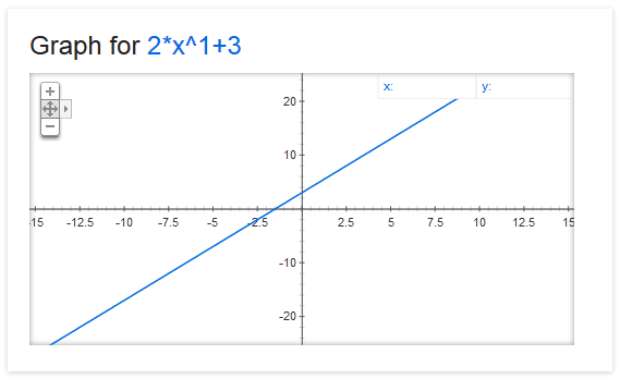
linearPolynomial.SetIndeterminateValue(argument, 0.0);

This way, the polynomial became a function: y = 2x + 3 (slope is 2.0, intercept is 3.0) and its value will be calculated for argument 0.0 (GetValue() method).

Full code of this example:

String slope = "a";
String intercept = "b";
String argument = "x";

// Declare all indeterminates and coefficients
Polynomial linearPolynomial = new Polynomial(
    new String[] { argument }
    , new String[] { slope, intercept });

// Add terms
linearPolynomial.AddTerm(slope, new Dictionary<String, Double>() { { argument, 1.0 } });
linearPolynomial.AddTerm(intercept);

// Set coefficients
linearPolynomial.SetCoefficientValue(slope, 2.0);
linearPolynomial.SetCoefficientValue(intercept, 3.0);

// Set the indeterminate
linearPolynomial.SetIndeterminateValue(argument, 0.0);

Console.WriteLine(String.Format("Your polynomial: {0}", linearPolynomial.ToString()));
Console.WriteLine(String.Format("Value for argument 0.0: {0}", linearPolynomial.GetValue()));

Output:

Your polynomial: a * x^1.00 + b
Value for argument 0.0: 3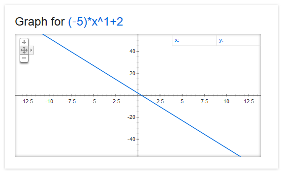

Similarly, our linear polynomial can be easily transformed into this function simply by changing its coefficients:

linearPolynomial.SetCoefficientValue(slope, -5.0);
linearPolynomial.SetCoefficientValue(intercept, 2.0);

Multivariate polynomials can easily represent planes like this one:

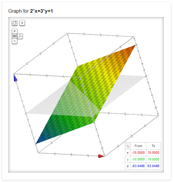
Source code:

String a = "a";
String b = "b";
String c = "c";
String x = "x";
String y = "y";

Polynomial linearPolynomial = new Polynomial(
    new String[] { x, y }
    , new String[] { a, b, c });

linearPolynomial.AddTerm(a, new Dictionary<String, Double>() { { x, 1.0 } });
linearPolynomial.AddTerm(b, new Dictionary<String, Double>() { { y, 1.0 } });
linearPolynomial.AddTerm(c);

linearPolynomial.SetCoefficientValue(a, 2.0);
linearPolynomial.SetCoefficientValue(b, 3.0);
linearPolynomial.SetCoefficientValue(c, 1.0);

linearPolynomial.SetIndeterminateValue(x, 1.0);
linearPolynomial.SetIndeterminateValue(y, 2.0);

Representing more complex functions is just a matter of adding more terms, indeterminates and coefficients. Let's take a look at this graph:

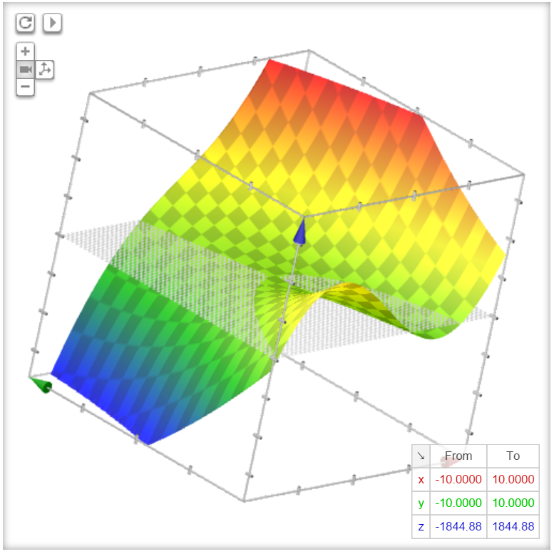
Source code:

String a = "a";
String b = "b";
String c = "c";
String d = "d";
String e = "e";
String x = "x";
String y = "y";

Polynomial linearPolynomial = new Polynomial(
    new String[] { x, y }
    , new String[] { a, b, c, d, e });

linearPolynomial.AddTerm(a, new Dictionary<String, Double>() { { x, 3.0 } });
linearPolynomial.AddTerm(b, new Dictionary<String, Double>() 
{ 
    { x, 1.0 }
    , { y, 1.0 } 
});
linearPolynomial.AddTerm(c, new Dictionary<String, Double>() { { y, 2.0 } });
linearPolynomial.AddTerm(d, new Dictionary<String, Double>() { { y, 1.0 } });
linearPolynomial.AddTerm(e);

linearPolynomial.SetCoefficientValue(a, 2.0);
linearPolynomial.SetCoefficientValue(b, 15.0);
linearPolynomial.SetCoefficientValue(c, 4.0);
linearPolynomial.SetCoefficientValue(d, 5.0);
linearPolynomial.SetCoefficientValue(e, 1.0);

linearPolynomial.SetIndeterminateValue(x, 1.0);
linearPolynomial.SetIndeterminateValue(y, 2.0);

This example shows how you can mix different indeterminates in one term.

If you face a situation where you have to use multiple structurally similar polynomials (let's say quadratic ones), differing only in the values of their coefficients, you don't have to create each one of them separately. You define your structure once, and then you can deep copy (Copy() method) it to create remaining polynomials. After you have a deep copy of your base polynomial, you can then assign desired values to each of the polynomial's coefficients.

If you want to compare polynomials, you have two methods at your disposal: Equals(Object obj) and Equals(Polynomial polynomialObject). The first one is just overridden .NET Equals and lets you compare your polynomials with virtually any object while the second one is more specialised and accepts only instances of the Polynomial class.

Comparison is divided into three stages: comparing the structure (quadratic polynomials should not be equal to the cubic ones), comparing the values of coefficients (2x + 3 is not 2x - 3) and comparing values of indeterminates (2x + 3 has different values for x = 1 and x = 2). If all of these conditions are met, polynomial are equal.