Code Monkey home page Code Monkey logo

shapviz's Introduction

{shapviz}

CRAN status R-CMD-check Codecov test coverage

Overview

{shapviz} provides typical SHAP plots:

  • sv_importance(): Importance plots (bar plots and/or beeswarm plots).
  • sv_dependence() and sv_dependence2D(): Dependence plots to study feature effects and interactions.
  • sv_interaction(): Interaction plots.
  • sv_waterfall(): Waterfall plots to study single predictions.
  • sv_force(): Force plots as alternative to waterfall plots.

SHAP and feature values are stored in a "shapviz" object that is built from:

  1. Models that know how to calculate SHAP values: XGBoost, LightGBM, h2o, or
  2. SHAP crunchers like {fastshap}, {kernelshap}, {treeshap}, {fastr}, {DALEX}, or simply from a
  3. SHAP matrix and its corresponding feature values.

Installation

# From CRAN
install.packages("shapviz")

# Or the newest version from GitHub:
# install.packages("devtools")
devtools::install_github("ModelOriented/shapviz")

Usage

Shiny diamonds... let's use XGBoost to model their prices by the four "C" variables:

library(shapviz)
library(ggplot2)
library(xgboost)

set.seed(1)

# Build model
x <- c("carat", "cut", "color", "clarity")
dtrain <- xgb.DMatrix(data.matrix(diamonds[x]), label = diamonds$price)
fit <- xgb.train(params = list(learning_rate = 0.1), data = dtrain, nrounds = 65)

# SHAP analysis: X can even contain factors
dia_2000 <- diamonds[sample(nrow(diamonds), 2000), x]
shp <- shapviz(fit, X_pred = data.matrix(dia_2000), X = dia_2000)

sv_importance(shp, show_numbers = TRUE)
sv_dependence(shp, v = x)

Decompositions of individual predictions can be visualized as waterfall or force plot:

sv_waterfall(shp, row_id = 1)
sv_force(shp, row_id = 1)

More to Discover

Check-out the vignettes for topics like:

  • How to work with other SHAP packages like {fastshap}, {kernelshap} or {treeshap}?
  • SHAP interactions.
  • Multiple models, multi-output models, and subgroup analyses.
  • Plotting geographic effects.

References

[1] Scott M. Lundberg and Su-In Lee. A Unified Approach to Interpreting Model Predictions. Advances in Neural Information Processing Systems 30 (2017).

shapviz's People

Contributors

adrianstando avatar jmaspons avatar kapsner avatar mayer79 avatar olivroy avatar

Stargazers

 avatar  avatar  avatar  avatar  avatar  avatar  avatar  avatar  avatar  avatar  avatar  avatar  avatar  avatar  avatar  avatar  avatar  avatar  avatar  avatar  avatar  avatar  avatar  avatar  avatar  avatar  avatar  avatar  avatar  avatar  avatar  avatar  avatar  avatar  avatar  avatar  avatar  avatar  avatar  avatar  avatar  avatar  avatar  avatar  avatar  avatar  avatar  avatar  avatar  avatar  avatar  avatar  avatar  avatar  avatar  avatar  avatar  avatar  avatar  avatar  avatar

Watchers

 avatar  avatar  avatar  avatar  avatar

shapviz's Issues

Odd findings in sv_importance() using beeswarm.

Hi

We have ran a analysis on a multiclass problem:

X = bake(prep(recipe), new_data = train_data)
X_pred = bake(prep(recipe), has_role("predictor"), new_data = train_data, composition = "matrix")


set.seed(2023)
SHAP_VIZ_Explainer <-shapviz::shapviz(object = tidymodels_final_model, X_pred = X_pred, X = X)


shapviz::sv_importance(object = SHAP_VIZ_Explainer, kind = "beeswarm", max_display  = 20, show_numbers = FALSE)

feature_importance_class_bee

The plot from above illustrates the biggest class of the three.

Two questions came up my mind:

  1. The third feature from top is a categorical feature with Yes and No. Both Yes and No are on the same side, for which we do not have an explanation.
  2. In multiple other features (mostly categorical), we see kind of a pattern of vertical lines. Could this pattern arose from correlations with other features?

We would highly appreciate your thoughts and interpretation of our findings.

issue with sv_importance function

Hi,
I am running you code and run into below error:

shapviz::sv_importance(shp)
Error in FUN(newX[, i], ...) : unused argument (simplify = FALSE)

Can you please help?

Multiclass/Multioutput/multiple models

Introduce class "mshapviz" that would combine multiple "shapviz" objects representing SHAP values from

  • multiple models,
  • a multi-class model (XGBoost, kernelshap), or
  • a multi-output regression (kernelshap).

Multiple "shapviz" objects could be combined to a "mshapviz" object by c(...) or mshapviz(...). Existing methods like [, +, rbind, colnames, dim would need to be written to cover "mshapviz" objects as well.

As a start, the sv_xyz() plot functions would use patchwork::wrap_plots(list). The resulting combined plot can be modified using &, e.g., & ylim(...). This gives quite some flexibility.

how to get Shap interactions for LightGBM?

Your package is great, and very easy to use within tidymodels framework. I was wondering if it is possible to calculate interactions for LightGBM. I would like to use that instead of the heuristic (which is an amazing solution tho) in sv_dependence. I've seen that for Xgboost is possible and there is a param Interaction = T to set in shapviz.base. Any solution workaround for LightGBM?

Multiple plots: align SHAP axis limits

It would be convenient to add a fixed_shap_axis = TRUE argument to sv_dependence().

When multiple plots are generated via {patchwork}, one typically wants to use a common SHAP axis (vertical axis). In the current documentation, this is done manually by passing & ylim(a, b). The argument fixed_shap_axis would deal with it automatically using some ggplot2 magic.

image

PS: A similar logic could be used in other plots as well, e.g., in sv_importance() etc. I think it is a bit more difficult there because their SHAP axis is already slightly modified. sv_interaction() should be as easy as sv_dependence(), but less important.

Make viridis arguments explicit

Currently, the color scale in sv_importance() and sv_dependence() can be controlled by an option. These functions should gain an explicit argument to overwrite this option.

Cannot rename colnames/dimnames in post-processing

Consider a simple force plot generated from the diamonds dataset:

library(shapviz)
library(ggplot2)
library(xgboost)

set.seed(3653)

x <- c("carat", "cut", "color", "clarity")
dtrain <- xgb.DMatrix(data.matrix(diamonds[x]), label = diamonds$price)
fit <- xgb.train(params = list(learning_rate = 0.1), data = dtrain, nrounds = 65)

# Explanation data
dia_small <- diamonds[sample(nrow(diamonds), 2000), ]

shp <- shapviz(fit, X_pred = data.matrix(dia_small[x]), X = dia_small)

sv_force(shp, row_id = 1)

image

Because I currently live in Europe, I would like to change the color=F in this plot to colour=F as in UK ortography.

> colnames(shp)
[1] "carat"   "cut"     "color"   "clarity"
> colnames(shp) <- c("carat", "cut", "colour", "clarity")
Error in dimnames(x) <- dn : 'dimnames' applied to non-array

Although the shapviz class defines an S3 method for colnames, there is no way to alter the colnames/dimnames because the class does not have array-like inheritance for the underlying matrix. Passing dimnames for both axes of the dimensions will also fail:

> dimnames(shp)
[[1]]
NULL

[[2]]
[1] "carat"   "cut"     "color"   "clarity"

> dimnames(shp) <- list(NULL, c("carat", "cut", "colour", "clarity"))
Error in dimnames(shp) <- list(NULL, c("carat", "cut", "colour", "clarity")) : 
  'dimnames' applied to non-array

Essentially, I want to be able to post-process the shapviz object for human readibility. Another use-case could be when working with categorical variables and using collapse (#7 ) where renaming variables before the shapviz object is generated might not be feasible.

Baseline-value question

Hey there!

Maybe I have missed it in the vignette, but what is the output of the get_baseline function? Is it the mean prediction of the model in the dataset you extract the shap values in the log-odds scale? For some reason I see some differences between the average prediction of my XGBoost model and the output of the get_baseline function (after I transform to probability). However, when I use the explain function from DALEX and plot the contributions for a single observation, then the E[f(x)] corresponds perfectly with the mean prediction of the model, as extracted from the explainer.

Thank you in advance!

Idea: sv_dependence2D()

What about a new scatterplot sv_dependence2D() as a way to study bivariate or interaction effects:

  • x and y coordinate represent two features, e.g. coordinates
  • Color scale represents the sum of their SHAP values
  • Optionally, the SHAP values of additional features (like distance to next train station) could be added to the sum
  • Multiple x xor y variables could be selected and shown via patchwork
  • If interaction =T, instead of the rowwise sum, SHAP interactions would be shown.

What geometry would look good? Jittered scatterplot? Or averages over binned feature values?

Remove dependency to ggbeeswarm

An important dependency, "ggbeeswarm", is at risk to be removed from CRAN. To reduce the dependency footprint of "shapviz", it would be a great first step to replace "ggbeeswarm" by native R code. This would also remove dependencies to "vipor" and "beeswarm".

Add collapsing logic

Related to: #7

The idea is to add a collapse argument to shapviz(). This is a named list specifying which groups of SHAP columns are to be collapsed by summation. This will allow to combine one-hot-encoded factors to a single one for explanation.

Add plots for SHAP interactions

XGBoost and treeshap package are able to provide SHAP values for pairwise interactions. The following plots could be considered:

It would be nice to see some useful plots for these. An idea would be to show

  • waterfall, force, importance plots where one could see which part comes from the main effect an which from the strongest few pairwise interactions.
  • Dependence plots maybe like SHAP package in Python?

SHAP aggregates

Like SHAP aggregate value in {DALEX},

  • sv_waterfall()
  • sv_force()

should be able to act on multiple observations. In this case, their SHAP values and predictions would be averaged. Feature values would be shown only if unique.

Probabiliy on x-axis for a class

I am doing a classification task using xgboost. When calculating values with shapviz, is it possible to somehow scale the SHAP value into the scale of the probability of one of the two classes in a binary classification problem?

sv_importance returns unused argument error

Calling sv_importance results in:

Error in FUN(newX[, i], ...) : unused argument (simplify = FALSE)

Looking through shapviz/tree/main/R)/sv_importance.R; the .min_max_scale helper function indeed does not include the simplify argument,

repro steps as in the shapviz vignette

X_train_test <- data.matrix(iris[, -1])
dtrain_test <- xgboost::xgb.DMatrix(X_train_test, label = iris[, 1])
fit_test <- xgboost::xgb.train(data = dtrain_test, nrounds = 50)
x_test <- shapviz(fit_test, X_pred = X_train_test)
sv_importance(x_test)
sv_importance(x_test, kind = "beeswarm", show_numbers = TRUE)

Note, the following works as intended:
sv_importance(x_test, kind = "no")

Cheers

Custom color palettes for the beeswarm plot

So changing the color options of the vivisdris package works for t
sv_importance(shp, kind = "beeswarm", viridis_args = list(begin = 0.0, end = 0.85, option = "mako"))
However, is it possible to change the colors manually using hex-codes (e.g. "#005f7f" and "#f34c7f" )?

(maybe using something similar to
ggplot(data, aes(x, y, fill = value)) + geom_tile() + scale_fill_gradientn(colors = c("#005f7f", "#f34c7f"), na.value = "transparent") + theme_minimal()
but I am not sure how to include this to the sv_importance code)

Color of the circle in the plotfrom `sv_dependence()`

Can you allow the color of the circle in the plot from sv_dependence() to be set to something other than purple, or even remove the color outline for the points on the plot? Like chart from SHAPforxgboost::shap.plot.dependence()

Best practice for visualizing tidymodels last_fit() object

Dear Authors,

I'm currently struggling with the shapviz explainer for tidymodels.
I've checked the examples provided for the diamond package using only fit() for the training data.

What would be your recommended best practices for visualizing the following two tidymodels objects:

1.) Results from workflow_map() using cv_resamples and tuning_grid using an xgboost model on training data

2.) Results from last_fit() using the best model from 1.)

Thanks in advance for your suggestions.

Beeswarm plot: Connecting visualisations to waterfall-style plots

Today, I was working with a colleague. I explained how the waterfall plot has the advantage of focussing on a single entry, where the beeswarm plot offers a summary of the model. He then asked, if it would somehow be possible to combine the two:

  • A beeswarm plot
  • But showing where a single entry lands in the clouds of datapoints

Below is a mock-up of what this could look like:

sv_importance(shp, kind = "beeswarm", row_id = 1)

image

sv_importance could take an additional param row_id to highlight the corresponding data points for the nth row of SHAP values, similar to waterfall and force. I don't think there is much freedom in color-choice here (if we want to make something colorblind-friendly), so maybe arrows and labels could be used to point at the approx. location of values.

Sound meaningful?

linewidth aesthetic ggplot

In ggplot2 version 3.4, the "size" aesthetic in line-based geoms have been replaced by "linewidth".

  • Will need to replace "size" by "linewidth" in sv_waterfall() and sv_force().
  • Will need to add min version of ggplot2 to 3.4

Cannot set x-axis limits with beeswarm plot when data exist outside of specified xlims

I would like to trim the x-axis of a shap beeswarm plot to a specified range using ggplot2::xlim(). If I use xlims that are greater than the min or less than the max shap value, then there is an error from the stats::density.default function, which is used for kernel density estimation.

Error in `ggplot2::geom_point()`:
! Problem while computing position.
ℹ Error occurred in the 2nd layer.
Caused by error in `density.default()`:
! 'x' contains missing values

The 2nd layer is xlim(, )

The lines throwing the error in density.default are:

x.na <- is.na(x)
    if (any(x.na)) {
        if (na.rm) 
            x <- x[!x.na]
        else stop("'x' contains missing values")
    }

There are no NA values in my shap dataframe, so I think the NA are introduced from the xlim(). So, I think the beeswarm plot needs to be edited to handle this case. Or is there another way to trim the x-axis?

There is no issue trimming the barplot.

maintenance: changes in package_version()

CRAN informed that package_version() will stop to accept numeric values (for good reasons).

This row should be fixed accordingly:

utils::packageVersion("lightgbm") >= 4

Upcoming changes to fastshap

Thanks for this awesome package. I've decided to deprecate the hacky plotting functions in fastshap in favor of using this package. However, a couple of upcoming changes in v0.8.0 might require some minor changes to the shapviz.explain() method. In short:

  • The explain() function essentially returns a matrix now, as opposed to a tibble.
  • The output from explain() now also contains a "baseline" attribute, which could be useful to default to in some of the plotting functions.

Looking to update on CRAN sometime mid-November.

Separate SHAP summary and SHAP importance plots

Currently, sv_importance() can plot both bar plots with SHAP importances and SHAP summary plots (= beeswarm plots of SHAP values, colored by normalized feature values).

We should separate the two things into

  • sv_importance() showing a bar plot with option plot = TRUE to cover kinds "bar" and "no".
  • sv_summary() showing a beeswarm plot with option show_bars = FALSE to cover kinds "bee" and "both".

This will give the necessary flexibility to think about SHAP interactions.

The process will be as follows:

  1. Moving the code of sv_importance() to a helper function f() basically equaling to sv_importance().
  2. Add sv_summary() pointing to f().
  3. Let sv_importance() point to f() and showing a depreciation warning that kind = bee/both will be removed in the next major release.
  4. Separate the functionality of f() to each of the two main functions.

Better default for sv_importance()

The default plot for sv_importance() should be a bar plot rather than a beeswarm plot. There are different reasons:

  • It is easier to grasp
  • It is faster to compute
  • Having in mind future plots for SHAP interaction, some type of bar plot is more realistic than an adaption of the beeswarm plot

{lightgbm} v4.0.0 is coming

👋 hey @mayer79 !

As you know from discussions we've had over in https://github.com/microsoft/LightGBM, at {lightgbm} has been accumulating breaking changes in preparation for a v4.0.0 release (microsoft/LightGBM#5153).

To make up for the fact that so many of these changes are being released directly without a deprecation cycle (microsoft/LightGBM#5133 (comment)), I'm willing to come here and contribute fixes to make {shapviz} compatible with both older and newer versions of {lightgbm}.

Are you open to such contributions?

I'd also be happy to document here in this issue how you and anyone contributing to this project can test it against the development version of LightGBM, if you think that'd help. (e.g., as I did here for {bonsai}: tidymodels/bonsai#34 (comment)).

Thanks so much for all your contributions to LightGBM and for maintaining this package that allows people to get more information out of their LightGBM models!

Interaction importance

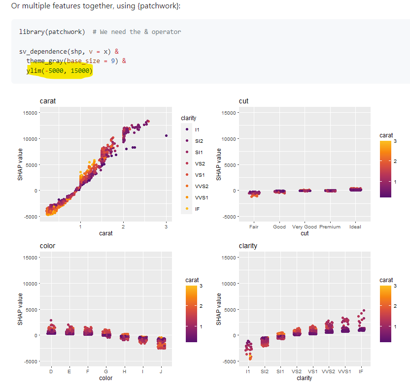
I think it would be useful to have a function that computes/visualises the relative importance of interaction effects.

Here's an example for an xgboost model where SHAP interaction values are available:

library(shapviz)
library(tidyverse)
library(xgboost)

set.seed(3653)
x <- c("carat", "cut", "color", "clarity")
dtrain <- xgb.DMatrix(data.matrix(diamonds[x]), label = diamonds$price)
fit <- xgb.train(params = list(learning_rate = 0.1), data = dtrain, nrounds = 65)

# Explanation data
dia_small <- diamonds[sample(nrow(diamonds), 2000), ]

# shapviz object with SHAP interaction values
shp_i <- shapviz(
  fit, X_pred = data.matrix(dia_small[x]), X = dia_small, interactions = TRUE
)

# Interaction importance
shap_interactions <- apply(2 * abs(shp_i$S_inter), c(2, 3), mean)
shap_interactions[lower.tri(shap_interactions, diag = TRUE)] <- NA
as.data.frame.table(shap_interactions, responseName = "interaction_strength") %>% 
  filter(!is.na(interaction_strength)) %>% 
  arrange(desc(interaction_strength))
#>    Var1    Var2 interaction_strength
#> 1 carat clarity            600.07087
#> 2 carat   color            412.44253
#> 3 color clarity            188.35864
#> 4 carat     cut             98.98317
#> 5   cut clarity             23.92846
#> 6   cut   color             17.94669

Created on 2023-10-24 with reprex v2.0.2

Ideally, this function would also work, based on some heuristics, for models that don't have SHAP interaction values available. I don't think using the heuristics in potential_interactions() (weighted squared correlations) willl work here as it doesn't take the amount of variation of the SHAP values in each bin into account, so the current interaction importance values are not comparable across features.

Maybe switching to the modelled part of the variation would work (and note that this also addresses #119): in each bin, fit a linear regression model and compute the mean of the absolute values of the fitted values minus the overall mean. I believe this boils down to the SHAP importance metric for a linear regression model with one feature. Doing so brings it on a scale that's comparable across bins and across features (differente vs in potential_interactions()).

Here's a code example to illustrate what I mean more clearly:

# shapviz object without interactions
shp <- shapviz(
  fit, X_pred = data.matrix(dia_small[x]), X = dia_small, interactions = FALSE
)

# Replace correlation measure with modelled variation measure
# Swapping out the function `r_sq` with `mod_var` 
potential_interactions_modelled <- function(obj, v) {
  stopifnot(is.shapviz(obj))
  S <- get_shap_values(obj)
  S_inter <- get_shap_interactions(obj)
  X <- get_feature_values(obj)
  nms <- colnames(obj)
  v_other <- setdiff(nms, v)
  stopifnot(v %in% nms)
  
  if (ncol(obj) <= 1L) {
    return(NULL)
  }
  
  # Simple case: we have SHAP interaction values
  if (!is.null(S_inter)) {
    return(sort(2 * colMeans(abs(S_inter[, v, ]))[v_other], decreasing = TRUE))
  }
  
  # Complicated case: we need to rely on modelled variation based heuristic
  mod_var <- function(s, x) {
    sapply(x, 
           function(x) {
             tryCatch({
               mean(abs(stats::lm(s ~ x)$fitted - mean(s)))
             }, error = function(e) {
               return(NA)
             })
           })
  }
  n_bins <- ceiling(min(sqrt(nrow(X)), nrow(X) / 20))
  v_bin <- shapviz:::.fast_bin(X[[v]], n_bins = n_bins)
  s_bin <- split(S[, v], v_bin)
  X_bin <- split(X[v_other], v_bin)
  w <- do.call(rbind, lapply(X_bin, function(z) colSums(!is.na(z))))
  modelled_variation <- do.call(rbind, mapply(mod_var, s_bin, X_bin, SIMPLIFY = FALSE))
  sort(colSums(w * modelled_variation, na.rm = TRUE) / colSums(w), decreasing = TRUE)
}

# Current implementation with SHAP interaction values
potential_interactions(shp_i, v = "cut")
#>    carat  clarity    color 
#> 98.98315 23.92846 17.94669

# Current implementation based on heuristics 
potential_interactions(shp, v = "cut")
#>      carat    clarity      color 
#> 0.49739669 0.07223855 0.04243011

# Suggested implementation based on heuristics 
potential_interactions_modelled(shp, v = "cut")
#>    carat  clarity    color 
#> 35.23818 14.73922 10.66934

# Current implementation with SHAP interaction values
potential_interactions(shp_i, v = "carat")
#>   clarity     color       cut 
#> 600.07087 412.44253  98.98317

# Current implementation based on heuristics 
potential_interactions(shp, v = "carat")
#>   clarity     color       cut 
#> 0.5301601 0.1545190 0.1121987

# Suggested implementation based on heuristics 
potential_interactions_modelled(shp, v = "carat")
#>  clarity    color      cut 
#> 248.3854 177.3795 132.6098

# Function to create table with ranked interaction variables
table_potential_interactions <- function(predictor) {
  pi <- potential_interactions_modelled(shp, predictor)
  tibble(var1 = predictor, var2 = names(pi), interaction_strength = pi)
}

# Interaction importance
map(x, table_potential_interactions) %>% 
  bind_rows() %>% 
  arrange(desc(interaction_strength))
#> # A tibble: 12 × 3
#>    var1    var2    interaction_strength
#>    <chr>   <chr>                  <dbl>
#>  1 carat   clarity                248. 
#>  2 clarity carat                  186. 
#>  3 carat   color                  177. 
#>  4 carat   cut                    133. 
#>  5 color   carat                  128. 
#>  6 clarity color                   89.3
#>  7 color   clarity                 55.6
#>  8 clarity cut                     48.7
#>  9 cut     carat                   35.2
#> 10 color   cut                     25.0
#> 11 cut     clarity                 14.7
#> 12 cut     color                   10.7

Note that this analysis is not symmetric, but I don't think that's an issue as the table above is informative: it suggests you to split out var1 effects by var2 and hence look at PD plots or SHAP dependence plots for var1 by different segments of var2.

Multioutput model names

Upon construction of a "mshapviz" object, class names or other response names are lost. This should be fixed.

Not compatible with mlr3 package and DALEXtra package

Thanks to your shapviz package, we can do many beautiful visualizations of shap values in the R environment. Since there are many current machine learning algorithms, everyone tends to use a system with a unified wrapper, such as mlr3. Your shapviz package can construct shapviz objects using the results of the predict_parts function of the DALEXtra package. The DALEXtra package can also build an explainer for the results of mlr3 for the next step of predict_parts calculation. However, I found some problems when applying the above process in practice.

`

Create explainer from your mlr3 model

titanic_imputed$survived <- as.factor(titanic_imputed$survived)
task_classif <- TaskClassif$new(id = "1", backend = titanic_imputed, target = "survived")
learner_classif <- lrn("classif.rpart", predict_type = "prob")
learner_classif$train(task_classif)
exp3<- explain_mlr3(learner_classif, data = titanic_imputed,
y = as.numeric(as.character(titanic_imputed$survived)))

Instance Level shap of the Model Predictions

pred_part3<- DALEX::predict_parts(explainer = exp3,
new_observation = titanic_imputed[,1:7],
type = "shap")

Initialize "shapviz" Object

sv <- shapviz(pred_part3)

SHAP Importance Plots

sv_importance(sv,kind = "beeswarm")`

image

Random Forests

Is there a way to get this to also work with random forest models?

Individual baselines

The "shap" package in Python stores baseline values per observation, while {shapviz} stores a single value. In most of the cases, this will do the job, but the Python logic is more flexible.

We should probably switch to the more flexible solution. A lot of functions need to be adapted, but the change affects only two plot functions: sv_force() and sv_waterfall(). The other functions do not need a baseline.

See also the discussion here: #111 (comment)

Override or transform label values

The default behaviour of sv_waterfall and sv_forceplot is to print out the associated value for a given attribute:
image

This is good, but a bit confusing when working with pre-processed data (f.x. normalised values). It would be very nice if the labels could be overridden or "transformed" in the final plot.

Deprecate "show_others" in sv_importance()

If there are many features, sv_importance() uses a complicated collapse logic per default.

  • A better default is to just show the top m features, without an "other" category.
  • To simplify the code, we can deprecate the old default.

Controlling threads

How to control the number of threads used by XGBoost (and most probably its dependency data.table)?

In CRAN submissions, I got

* checking tests ... [41s/4s] NOTE
  Running ‘testthat.R’ [41s/4s]
Running R code in ‘testthat.R’ had CPU time 9.4 times elapsed time

Similar for examples.

Consequence:

  • All examples -> dontrun
  • All unit tests using XGBoost commented out -> low test coverage

There are discussions on the R dev mailing list that CRAN might limit resources per package from their side. But of course, it would be great to fix the problem already now.

What I have tried:

  1. Set params = list(nthread = 1) in all XGBoost tests
  2. Set nrounds = 1 in all XGBoost tests
  3. Set environment variables in the test script before loading {shapviz}. I think this does not work because the session has already started at that moment.
  4. Set `data.table::setDTthreads(1) in the test script.

Any hints?

Similar To Log Odds Plot

Is it possible to create something like this but with SHAP values? Something like the bee swarm plot, but one that looks more in use by statistics? The points are determined by using a logistic regression, and each point represents the estimate of a certain covariate (feature) having an effect via a change in log odds of event of interest occurring.

image

Treatment of categorical features in `potential_interactions()`: suggestion to use R squared instead of squared correlation

Thanks for providing a great SHAP visualisation package for R!

I'm looking into fast ways to surface interaction effects in H2O GBMs. Unfortunately, unlike xgboost, H2O does not provide interaction SHAP values and hence shapviz relies on a heuristic based on weighted squared Pearson correlation between the SHAP value and other features' values in its potential_interactions() implementation. I think that's a reasonable approach, but it doesn't work well for unordered categorical features (where it converts them to their arbitrarily ordered factor level numbers using data.matrix()).

A natural extension of what you are doing now, which I believe would be more appropriate for categorical features, would be to consider the R squared of a linear regression model of the SHAP values on each of the other feature. For continuous features, that would give you the exact same value you have now. For categorical features, that would be measuring the association between the unordered factor levels and the SHAP values in a way that's not constraint by the arbitrary feature level numbering.

If you want to implement that, lines 230-233 would have to be replaced by:

  # Complicated case: we need to rely on R squared based heuristic
  r_sq <- function(s, x) {
    sapply(x, 
           function(x) {
             tryCatch({
               summary(stats::lm(s ~ x))$r.squared
             }, error = function(e) {
               return(NA)
             })
           })
  }

Here's a full example using a public H2O data set:

library(shapviz)
library(h2o)
h2o.init()

# Import the prostate dataset into H2O:
prostate <- h2o.importFile("http://s3.amazonaws.com/h2o-public-test-data/smalldata/prostate/prostate.csv")

# Set the predictors and response; set the factors:
prostate$CAPSULE <- as.factor(prostate$CAPSULE)
prostate$RACE <- as.factor(prostate$RACE)
prostate$DPROS <- as.factor(prostate$DPROS)
prostate$DCAPS <- as.factor(prostate$DCAPS)
prostate$GLEASON <- as.factor(prostate$GLEASON)
predictors <- c("AGE", "RACE", "DPROS", "DCAPS", "PSA", "VOL", "GLEASON")
response <- "CAPSULE"

# Build and train the model:
pros_gbm <- h2o.gbm(x = predictors,
                    y = response,
                    nfolds = 5,
                    seed = 1111,
                    keep_cross_validation_predictions = TRUE,
                    training_frame = prostate)

# Create shapviz object
shp <- shapviz(pros_gbm, X_pred = prostate, X = as.data.frame(prostate))

# Replace correlation measure with R squared measure
potential_interactions_rsq <- function(obj, v) {
  stopifnot(is.shapviz(obj))
  S <- get_shap_values(obj)
  S_inter <- get_shap_interactions(obj)
  X <- get_feature_values(obj)
  nms <- colnames(obj)
  v_other <- setdiff(nms, v)
  stopifnot(v %in% nms)
  
  if (ncol(obj) <= 1L) {
    return(NULL)
  }
  
  # Simple case: we have SHAP interaction values
  if (!is.null(S_inter)) {
    return(sort(2 * colMeans(abs(S_inter[, v, ]))[v_other], decreasing = TRUE))
  }
  
  # Complicated case: we need to rely on R squared based heuristic
  r_sq <- function(s, x) {
    sapply(x, 
           function(x) {
             tryCatch({
               summary(stats::lm(s ~ x))$r.squared
             }, error = function(e) {
               return(NA)
             })
           })
  }
  n_bins <- ceiling(min(sqrt(nrow(X)), nrow(X) / 20))
  v_bin <- shapviz:::.fast_bin(X[[v]], n_bins = n_bins)
  s_bin <- split(S[, v], v_bin)
  X_bin <- split(X[v_other], v_bin)
  w <- do.call(rbind, lapply(X_bin, function(z) colSums(!is.na(z))))
  cor_squared <- do.call(rbind, mapply(r_sq, s_bin, X_bin, SIMPLIFY = FALSE))
  sort(colSums(w * cor_squared, na.rm = TRUE) / colSums(w), decreasing = TRUE)
}

# Current implementation
potential_interactions(shp, v = "PSA")
#>    GLEASON      DPROS        VOL      DCAPS       RACE        AGE 
#> 0.14827267 0.10383619 0.07988404 0.07166984 0.06715848 0.05922560

# Suggested implementation
potential_interactions_rsq(shp, v = "PSA")
#>    GLEASON      DPROS        VOL       RACE      DCAPS        AGE 
#> 0.32998601 0.25517234 0.07988404 0.07827180 0.07166984 0.05922560

Created on 2023-10-24 with reprex v2.0.2

Recommend Projects

  • React photo React

    A declarative, efficient, and flexible JavaScript library for building user interfaces.

  • Vue.js photo Vue.js

    🖖 Vue.js is a progressive, incrementally-adoptable JavaScript framework for building UI on the web.

  • Typescript photo Typescript

    TypeScript is a superset of JavaScript that compiles to clean JavaScript output.

  • TensorFlow photo TensorFlow

    An Open Source Machine Learning Framework for Everyone

  • Django photo Django

    The Web framework for perfectionists with deadlines.

  • D3 photo D3

    Bring data to life with SVG, Canvas and HTML. 📊📈🎉

Recommend Topics

  • javascript

    JavaScript (JS) is a lightweight interpreted programming language with first-class functions.

  • web

    Some thing interesting about web. New door for the world.

  • server

    A server is a program made to process requests and deliver data to clients.

  • Machine learning

    Machine learning is a way of modeling and interpreting data that allows a piece of software to respond intelligently.

  • Game

    Some thing interesting about game, make everyone happy.

Recommend Org

  • Facebook photo Facebook

    We are working to build community through open source technology. NB: members must have two-factor auth.

  • Microsoft photo Microsoft

    Open source projects and samples from Microsoft.

  • Google photo Google

    Google ❤️ Open Source for everyone.

  • D3 photo D3

    Data-Driven Documents codes.