Label-free Cell segmentation is classifying a microscopic image area, pixels representing individual cell instances. It is a fundamental step in many biomedical studies and needs to be meticulously processed.

It is a process that helps the biologist quickly notice the background from the foreground in the cell segmentation task, categorizing pixels into significant regions. Cell segmentation is crucial for biologists to extract cells' morphology, polarity and motility. It increases the accuracy and speed of the diagnosis. It is also more robust and provides reliable results for biologists to use. This study compared ML and DL semantic segmentation methods for cancer cells in various environments.

• Data
• Semantic Segmentation with Traditional Machine Learning Methods
• Semantic Segmentation with Deep Learning Methods
• Analyzes
• References

Data Source: TUBITAK 119E578 Cell Motility Phase Contrast Time Lapse Microscopy Data-Set

The cells are examined in 3 different environments: matrigel, normal and collagen-coated. In experiments with a glass surface, the cells do not attach to the glass for long periods, and In most experiments, they are circular and shiny. On the other hand, matrigel-coated surfaces allow the cells to attach to the environment immediately. The collagen-coated also ensures a fast stick of cells such as matrigel. They are very different visually since they are different surfaces from each other.

Deep learning models are known to require large data sets for the training process. Unfortunately, we often need more data to be collected for a pixel classification problem. For example, collecting many biomedical images with your mobile phone is impossible. And then there's the label-up part, which needs to be more for an ordinary eye. Expert eyes and experience are required. But will ML algorithms surpass DL algorithms in a relatively shallow data set?

For each pixel, features are extracted using LBP, Haralick and 2D filters. Each pixel is then semantically classified by various ML methods.

Figure 1.1.1: The first step in constructing a LBP is to take the 8 pixel neighborhood surrounding a center pixel and threshold it to construct a set of 8 binary digits.

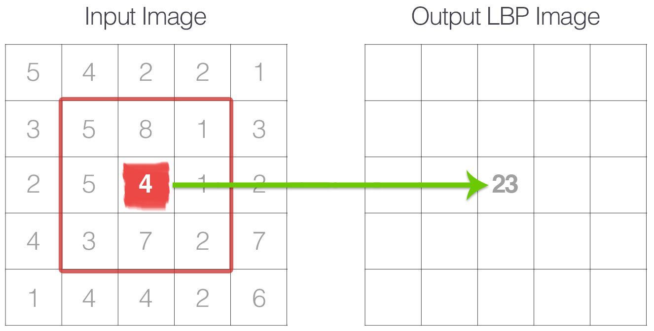
Figure 1.1.2: Taking the 8-bit binary neighborhood of the center pixel and converting it into a decimal representation.

Figure 1.1.3: Three neighborhood examples with varying p and r used to construct Local Binary Patterns.

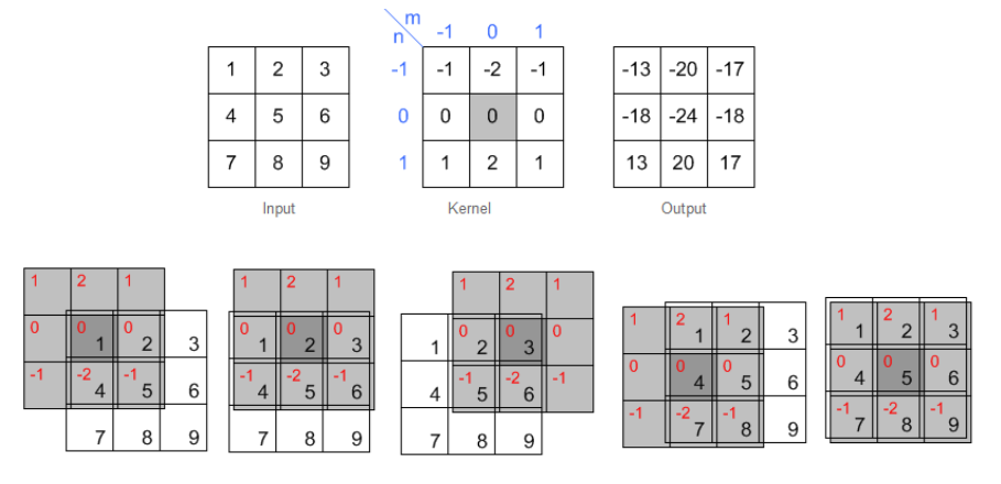
Figure 1.2.1: Example of 2D spatial filtering.

Figure 1.3.1: A description of how Haralick’s texture features are calculated. In an example 4 × 4 image ROI, three gray levels are represented by numerical values from 1 to 3. The GLCM is constructed by considering the relation of each voxel with its neighborhood. In this example we only look at the neighbor to the right. The GLCM acts like a counter for every combination of gray level pairs in the image. For each voxel, its value and the neighboring voxel value are counted in a specific GLCM element. The value of the reference voxel determines the column of the GLCM and the neighbor value determines the row. In this ROI, there are two instances when a reference voxel of 3 “co-occurs” with a neighbor voxel of 2, indicated in solid blue, and there is one instance of a reference voxel of 3 with a neighbor voxel of 1, indicated in dashed red. The normalized GLCM represents the frequency or probability of each combination to occur in the image. The Haralick texture features are functions of the normalized GLCM, where different aspects of the gray level distribution in the ROI are represented. For example, diagonal elements in the GLCM represent voxels pairs with equal gray levels. The texture feature “contrast” gives elements with similar gray level values a low weight but elements with dissimilar gray levels a high weight. It is common to add GLCMs from opposite neighbors (e.g. left-right or up-down) prior to normalization. This generates symmetric GLCMs, since each voxel has been the neighbor and the reference in both directions. The GLCMs and texture features then reflect the “horizontal” or “vertical” properties of the image. If all neighbors are considered when constructing the GLCM, the texture features are direction invariant.

Textural Features

1. Angular Second Moment

$f_1=Σ_iΣ_j{{p(i,j)}}^2$

2. Contrast

$f_2=Σ_{n=0}^{N_{g-1}} n^2(Σ_{i=1}^{N_g} Σ_{j=1}^{N_g}p(i,j))$

3. Correlation

$f_3=\frac{Σ_iΣ_j(ij)p(i,j)-\mu_x\mu_y}{\sigma_x\sigma_y}$

4. Variance

$f_4=Σ_iΣ_j(i-μ)^2p(i,j)$

5. Inverse Difference Moment

$f_5=Σ_iΣ_j\frac{1}{1+(i-j)^2}p(i,j)$

6. Sum Average

$f_6=Σ_{i=2}^{2N_g}ip_{x+y}(i)$

7. Sum Varience

$f_7=Σ_{i=2}^{2N_g}(i-f_8)^2p_{x+y}(i)$

8. Sum Entropy

$f_8=-Σ_{i=2}^{2N_g}p_{x+y}(i)log{(p_{x+y}(i))}$

9. Entropy

$f_9=Σ_iΣ_jp(i,j)log{(p(i,j))}$

10. Difference Varience

$f_{10}=varience:of:p_{x-y}$

11. Difference Entropy

$f_{11}=-Σ_{i=0}^{N_{g-1}}p_{x-y}(i)log{(p_{x-y}(i))}$

12. Information Features of Correlation

$f_{12}=\frac{HXY-HXY1}{max(HX,HY)}$, $f_{13}=(1-exp[-2(HXY2-HXY)])^\frac{1}{2}$, $HXY=-Σ_iΣ_jp(i,j)log{(p(i,j))}$, $HXY1=-Σ_iΣ_jp(i,j)log{(p_x(i)p_y(j))}$, $HXY2=-Σ_iΣ_jp_x(i)p_y(j)log{(p_x(i)p_y(j))}$

For DL methods, UNet [1], LinkNet [2] and PSPNet [3] were used.

Unet

LinkNet

PSPNet

DL approaches are pretty successful from ML approaches both numerically and visually.

But the ML algorithms performed relatively well. So ML algorithms can be a quick solution to save the day on even fewer data sets.

[1] Ronneberger, O., Fischer, P., & Brox, T. (2015, October). U-net: Convolutional networks for biomedical image segmentation. In International Conference on Medical image computing and computer-assisted intervention (pp. 234-241). Springer, Cham.

[2] Chaurasia, A., & Culurciello, E. (2017, December). Linknet: Exploiting encoder representations for efficient semantic segmentation. In 2017 IEEE Visual Communications and Image Processing (VCIP) (pp. 1-4). IEEE.

[3] Lin, T. Y., Dollár, P., Girshick, R., He, K., Hariharan, B., & Belongie, S. (2017). Feature pyramid networks for object detection. In Proceedings of the IEEE conference on computer vision and pattern recognition (pp. 2117-2125).

[4] LBP (Local Binary Patterns)

[5] R. M. Haralick, K. Shanmugam and I. Dinstein, "Textural Features for Image Classification," in IEEE Transactions on Systems, Man, and Cybernetics, vol. SMC-3, no. 6, pp. 610-621, Nov. 1973, doi: 10.1109/TSMC.1973.4309314.