insomnia's Introduction
insomnia's People
Contributors

Stargazers
insomnia's Issues
Decorators in python
Python data structures
Reading and writing files in python
postgresql tutorial
Install postgres
$ sudo apt update
$ sudo apt install postgresql postgresql-contrib
Switching over to the postgres account
$ sudo -u postgres psql
List all the commands
\?
List all the databases
\l
Connect to database
\c [DATABASENAME]
list tables, views, and sequences
Once connected you can check the database tables or schema by:
(options: S = show system objects, + = additional detail)
\d [S+]
List tables
\dt [PATTERN]
If want to see schema tables
\dt+
If you want to see specific schema tables
\dt schema_name.*
list table, view, and sequence access privileges
\dp
Quit postgres
\q
Create database
CREATE DATABASE [DATABASENAME];
Create table
CREATE TABLE [TABLENAME] (
    [COLUMNANEM1],
    [COLUMNANEM2],
    ...
);
Example:
CREATE TABLE playground (
    equip_id serial PRIMARY KEY,
    type varchar (50) NOT NULL,
    color varchar (25) NOT NULL,
    location varchar(25) check (location in ('north', 'south', 'west', 'east', 'northeast', 'southeast', 'southwest', 'northwest')),
    install_date date
);
Insert columns to table
INSERT INTO [TABLENAME]([COLUMN1], [COLUMN2], ...) VALUES([VALUE1], [VALUE2], ...) ;
Example:
INSERT INTO playground (type, color, location, install_date) VALUES ('slide', 'blue', 'south', '2017-04-28')
Select columns from table
SELECT [COLUMN(s)] FROM [TABLENAME];
Example:
SELECT * FROM playground;
Updating Data in a Table
UPDATE [TABLENAME] SET [COLUMNNSME=VALUE] WHERE [CONDITION(s)];
Example:
UPDATE playground SET color = 'red' WHERE type = 'swing';
Delete columns from table
DELETE FROM [TABLENAME] WHERE [CONDITION(s)];
Example:
DELETE FROM playground WHERE type = 'slide';
Adding columns to a table
ALTER TABLE [TABLENAME] ADD [COLUMN(s)];
Example:
ALTER TABLE playground ADD last_maint date;
Deleting columns from a table
ALTER TABLE [TABLENAME] DROP [COLUMN(s)];
Example:
ALTER TABLE playground DROP last_maint;
Drop table(s)
DROP TABLE [ IF EXISTS ] [TABLENAME] [, ...] [ CASCADE | RESTRICT ];
Example:
DROP TABLE [IF EXISTS] ;
Drop a database
#Change to postgres database
\c postgres
DROP DATABASE [IF EXISTS] [DATABASENAME];
Python string formatting
Classes in python
https://docs.python.org/3.6/tutorial/classes.html#classes
Introduction
Classes provide a means of bundling data and functionality together. Creating a new class creates a new type of object, allowing new instances of that type to be made. Each class instance can have attributes attached to it for maintaining its state. Class instances can also have methods (defined by its class) for modifying its state.
Python scopes and namespaces
Class Definition Syntax
The simplest form of class definition looks like this:
class ClassName:
    <statement-1>
    .
    .
    .
    <statement-N>
Python control statements
if Statements
Perhaps the most well-known statement type is the if statement. For example:
>>> x = int(input("Please enter an integer: "))
Please enter an integer: 42
>>> if x < 0:
...     x = 0
...     print('Negative changed to zero')
... elif x == 0:
...     print('Zero')
... elif x == 1:
...     print('Single')
... else:
...     print('More')
...
There can be zero or more elif parts, and the else part is optional. The keyword ‘elif’ is short for ‘else if’, and is useful to avoid excessive indentation. An if … elif … elif … sequence is a substitute for the switch or case statements found in other languages.
for Statements
The for statement in Python differs a bit from what you may be used to in C or Pascal. Rather than always iterating over an arithmetic progression of numbers (like in Pascal), or giving the user the ability to define both the iteration step and halting condition (as C), Python’s for statement iterates over the items of any sequence (a list or a string), in the order that they appear in the sequence. For example (no pun intended):
>>> # Measure some strings:
... words = ['cat', 'window', 'defenestrate']
>>> for w in words:
...     print(w, len(w))
...
cat 3
window 6
defenestrate 12
The range() Function
If you do need to iterate over a sequence of numbers, the built-in function range() comes in handy. It generates arithmetic progressions:
>>> for i in range(5):
...     print(i)
...
0
1
2
3
4
The given end point is never part of the generated sequence; range(10) generates 10 values, the legal indices for items of a sequence of length 10. It is possible to let the range start at another number, or to specify a different increment (even negative; sometimes this is called the ‘step’):
range(5, 10)
   5, 6, 7, 8, 9

range(0, 10, 3)
   0, 3, 6, 9

range(-10, -100, -30)
  -10, -40, -70
To iterate over the indices of a sequence, you can combine range() and len() as follows:
>>>
>>> a = ['Mary', 'had', 'a', 'little', 'lamb']
>>> for i in range(len(a)):
...     print(i, a[i])
...
0 Mary
1 had
2 a
3 little
4 lamb
break and continue Statements, and else Clauses on Loops
Loop statements may have an else clause; it is executed when the loop terminates through exhaustion of the list (with for) or when the condition becomes false (with while), but not when the loop is terminated by a break statement. This is exemplified by the following loop, which searches for prime numbers:
>>>
>>> for n in range(2, 10):
...     for x in range(2, n):
...         if n % x == 0:
...             print(n, 'equals', x, '*', n//x)
...             break
...     else:
...         # loop fell through without finding a factor
...         print(n, 'is a prime number')
...
2 is a prime number
3 is a prime number
4 equals 2 * 2
5 is a prime number
6 equals 2 * 3
7 is a prime number
8 equals 2 * 4
9 equals 3 * 3
(Yes, this is the correct code. Look closely: the else clause belongs to the for loop, not the if statement.)
When used with a loop, the else clause has more in common with the else clause of a try statement than it does that of if statements: a try statement’s else clause runs when no exception occurs, and a loop’s else clause runs when no break occurs. For more on the try statement and exceptions, see Handling Exceptions.
The continue statement, also borrowed from C, continues with the next iteration of the loop:
>>> for num in range(2, 10):
...     if num % 2 == 0:
...         print("Found an even number", num)
...         continue
...     print("Found a number", num)
Found an even number 2
Found a number 3
Found an even number 4
Found a number 5
Found an even number 6
Found a number 7
Found an even number 8
Found a number 9
pass Statements
The pass statement does nothing. It can be used when a statement is required syntactically but the program requires no action. For example:
>>>
>>> while True:
...     pass  # Busy-wait for keyboard interrupt (Ctrl+C)
...
This is commonly used for creating minimal classes:
>>>
>>> class MyEmptyClass:
...     pass
...
Another place pass can be used is as a place-holder for a function or conditional body when you are working on new code, allowing you to keep thinking at a more abstract level. The pass is silently ignored:
>>>
>>> def initlog(*args):
...     pass   # Remember to implement this!
...
Defining Functions
We can create a function that writes the Fibonacci series to an arbitrary boundary:
>>> def fib(n):    # write Fibonacci series up to n
...     """Print a Fibonacci series up to n."""
...     a, b = 0, 1
...     while a < n:
...         print(a, end=' ')
...         a, b = b, a+b
...     print()
...
>>> # Now call the function we just defined:
... fib(2000)
0 1 1 2 3 5 8 13 21 34 55 89 144 233 377 610 987 1597
The keyword def introduces a function definition. It must be followed by the function name and the parenthesized list of formal parameters. The statements that form the body of the function start at the next line, and must be indented.
The first statement of the function body can optionally be a string literal; this string literal is the function’s documentation string, or docstring. (More about docstrings can be found in the section Documentation Strings.)
The execution of a function introduces a new symbol table used for the local variables of the function. More precisely, all variable assignments in a function store the value in the local symbol table; whereas variable references first look in the local symbol table, then in the local symbol tables of enclosing functions, then in the global symbol table, and finally in the table of built-in names. Thus, global variables and variables of enclosing functions cannot be directly assigned a value within a function (unless, for global variables, named in a global statement, or, for variables of enclosing functions, named in a nonlocal statement), although they may be referenced.
The actual parameters (arguments) to a function call are introduced in the local symbol table of the called function when it is called; thus, arguments are passed using call by value (where the value is always an object reference, not the value of the object). 1 When a function calls another function, a new local symbol table is created for that call.
A function definition introduces the function name in the current symbol table. The value of the function name has a type that is recognized by the interpreter as a user-defined function. This value can be assigned to another name which can then also be used as a function. This serves as a general renaming mechanism:
More on Defining Functions
It is also possible to define functions with a variable number of arguments. There are three forms, which can be combined.
Default Argument Values
The most useful form is to specify a default value for one or more arguments. This creates a function that can be called with fewer arguments than it is defined to allow. For example:
def ask_ok(prompt, retries=4, reminder='Please try again!'):
    while True:
        ok = input(prompt)
        if ok in ('y', 'ye', 'yes'):
            return True
        if ok in ('n', 'no', 'nop', 'nope'):
            return False
        retries = retries - 1
        if retries < 0:
            raise ValueError('invalid user response')
        print(reminder)
This function can be called in several ways:
giving only the mandatory argument: ask_ok('Do you really want to quit?')
giving one of the optional arguments: ask_ok('OK to overwrite the file?', 2)
or even giving all arguments: ask_ok('OK to overwrite the file?', 2, 'Come on, only yes or no!')
This example also introduces the in keyword. This tests whether or not a sequence contains a certain value.
The default values are evaluated at the point of function definition in the defining scope, so that
i = 5
def f(arg=i):
    print(arg)

i = 6
f()
will print 5.
** Important warning: ** The default value is evaluated only once. This makes a difference when the default is a mutable object such as a list, dictionary, or instances of most classes. For example, the following function accumulates the arguments passed to it on subsequent calls:
def f(a, L=[]):
    L.append(a)
    return L

print(f(1))
print(f(2))
print(f(3))
This will print

[1]
[1, 2]
[1, 2, 3]
If you don’t want the default to be shared between subsequent calls, you can write the function like this instead:
def f(a, L=None):
    if L is None:
        L = []
    L.append(a)
    return L
Keyword Arguments
Functions can also be called using keyword arguments of the form kwarg=value. For instance, the following function:
def parrot(voltage, state='a stiff', action='voom', type='Norwegian Blue'):
    print("-- This parrot wouldn't", action, end=' ')
    print("if you put", voltage, "volts through it.")
    print("-- Lovely plumage, the", type)
    print("-- It's", state, "!")
accepts one required argument (voltage) and three optional arguments (state, action, and type). This function can be called in any of the following ways:
parrot(1000)                                          # 1 positional argument
parrot(voltage=1000)                                  # 1 keyword argument
parrot(voltage=1000000, action='VOOOOOM')             # 2 keyword arguments
parrot(action='VOOOOOM', voltage=1000000)             # 2 keyword arguments
parrot('a million', 'bereft of life', 'jump')         # 3 positional arguments
parrot('a thousand', state='pushing up the daisies')  # 1 positional, 1 keyword
but all the following calls would be invalid:
parrot()                     # required argument missing
parrot(voltage=5.0, 'dead')  # non-keyword argument after a keyword argument
parrot(110, voltage=220)     # duplicate value for the same argument
parrot(actor='John Cleese')  # unknown keyword argument
In a function call, keyword arguments must follow positional arguments. All the keyword arguments passed must match one of the arguments accepted by the function (e.g. actor is not a valid argument for the parrot function), and their order is not important. This also includes non-optional arguments (e.g. parrot(voltage=1000) is valid too). No argument may receive a value more than once. Here’s an example that fails due to this restriction:
>>>
>>> def function(a):
...     pass
...
>>> function(0, a=0)
Traceback (most recent call last):
  File "<stdin>", line 1, in <module>
TypeError: function() got multiple values for keyword argument 'a'
When a final formal parameter of the form **name is present, it receives a dictionary (see Mapping Types — dict) containing all keyword arguments except for those corresponding to a formal parameter. This may be combined with a formal parameter of the form *name (described in the next subsection) which receives a tuple containing the positional arguments beyond the formal parameter list. (*name must occur before **name.) For example, if we define a function like this:
def cheeseshop(kind, *arguments, **keywords):
    print("-- Do you have any", kind, "?")
    print("-- I'm sorry, we're all out of", kind)
    for arg in arguments:
        print(arg)
    print("-" * 40)
    for kw in keywords:
        print(kw, ":", keywords[kw])
It could be called like this:
cheeseshop("Limburger", "It's very runny, sir.",
           "It's really very, VERY runny, sir.",
           shopkeeper="Michael Palin",
           client="John Cleese",
           sketch="Cheese Shop Sketch")
and of course it would print:
-- Do you have any Limburger ?
-- I'm sorry, we're all out of Limburger
It's very runny, sir.
It's really very, VERY runny, sir.
----------------------------------------
shopkeeper : Michael Palin
client : John Cleese
sketch : Cheese Shop Sketch
Note that the order in which the keyword arguments are printed is guaranteed to match the order in which they were provided in the function call.
Lambda Expressions
Small anonymous functions can be created with the lambda keyword. This function returns the sum of its two arguments: lambda a, b: a+b. Lambda functions can be used wherever function objects are required. They are syntactically restricted to a single expression. Semantically, they are just syntactic sugar for a normal function definition. Like nested function definitions, lambda functions can reference variables from the containing scope:
>>> def make_incrementor(n):
...     return lambda x: x + n
...
>>> f = make_incrementor(42)
>>> f(0)
42
>>> f(1)
43
The above example uses a lambda expression to return a function. Another use is to pass a small function as an argument:
>>>
>>> pairs = [(1, 'one'), (2, 'two'), (3, 'three'), (4, 'four')]
>>> pairs.sort(key=lambda pair: pair[1])
>>> pairs
[(4, 'four'), (1, 'one'), (3, 'three'), (2, 'two')]
Documentation Strings
Here are some conventions about the content and formatting of documentation strings.
The first line should always be a short, concise summary of the object’s purpose. For brevity, it should not explicitly state the object’s name or type, since these are available by other means (except if the name happens to be a verb describing a function’s operation). This line should begin with a capital letter and end with a period.
If there are more lines in the documentation string, the second line should be blank, visually separating the summary from the rest of the description. The following lines should be one or more paragraphs describing the object’s calling conventions, its side effects, etc.
The Python parser does not strip indentation from multi-line string literals in Python, so tools that process documentation have to strip indentation if desired. This is done using the following convention. The first non-blank line after the first line of the string determines the amount of indentation for the entire documentation string. (We can’t use the first line since it is generally adjacent to the string’s opening quotes so its indentation is not apparent in the string literal.) Whitespace “equivalent” to this indentation is then stripped from the start of all lines of the string. Lines that are indented less should not occur, but if they occur all their leading whitespace should be stripped. Equivalence of whitespace should be tested after expansion of tabs (to 8 spaces, normally).
Here is an example of a multi-line docstring:
>>>
>>> def my_function():
...     """Do nothing, but document it.
...
...     No, really, it doesn't do anything.
...     """
...     pass
...
>>> print(my_function.__doc__)
Do nothing, but document it.

    No, really, it doesn't do anything.
Function Annotations
Annotations are stored in the annotations attribute of the function as a dictionary and have no effect on any other part of the function. Parameter annotations are defined by a colon after the parameter name, followed by an expression evaluating to the value of the annotation. Return annotations are defined by a literal ->, followed by an expression, between the parameter list and the colon denoting the end of the def statement. The following example has a positional argument, a keyword argument, and the return value annotated:
def f(ham: str, eggs: str = 'eggs') -> str:
    print("Annotations:", f.__annotations__)
    print("Arguments:", ham, eggs)
    return ham + ' and ' + eggs

f('spam')
Python global variables
Python naming conventions
Coding conventions for the Python code comprising the standard library in the main Python distribution.
Mongodb tutorial
MongoDB is a cross-platform, document oriented database that provides, high performance, high availability, and easy scalability. MongoDB works on concept of collection and document.
Database
Database is a physical container for collections. Each database gets its own set of files on the file system. A single MongoDB server typically has multiple databases.
Collection
Collection is a group of MongoDB documents. It is the equivalent of an RDBMS table. A collection exists within a single database. Collections do not enforce a schema. Documents within a collection can have different fields. Typically, all documents in a collection are of similar or related purpose.
Document
A document is a set of key-value pairs. Documents have dynamic schema. Dynamic schema means that documents in the same collection do not need to have the same set of fields or structure, and common fields in a collection's documents may hold different types of data.
The following table shows the relationship of RDBMS terminology with MongoDB.
| RDBMS | MongoDB |
|---|---|
| Database | Database |
| Table | Collection |
| Tuple/Row | Document |
| column | Field |
Advantages of MongoDB
- Schema less
MongoDB is a document database in which one collection holds different documents. Number of fields, content and size of the document can differ from one document to another. - Structure of a single object is clear.
- No complex joins.
- Deep query-ability. MongoDB supports dynamic queries on documents using a document-based query language that's nearly as powerful as SQL.
- Conversion/mapping of application objects to database objects not needed.
- Uses internal memory for storing the (windowed) working set, enabling faster access of data.
- Ease of scale-out − MongoDB is easy to scale.
Data modelling
Data in MongoDB has a flexible schema.documents in the same collection. They do not need to have the same set of fields or structure, and common fields in a collection’s documents may hold different types of data.
Some considerations while designing Schema in MongoDB
- Design your schema according to user requirements.
- Combine objects into one document if you will use them together. Otherwise separate them (but make sure there should not be need of joins).
- Duplicate the data (but limited) because disk space is cheap as compare to compute time.
- Do joins while write, not on read.
- Optimize your schema for most frequent use cases.
- Do complex aggregation in the schema.
Example
Suppose a client needs a database design for his blog/website and see the differences between RDBMS and MongoDB schema design. Website has the following requirements.
- Every post has the unique title, description and url.
- Every post can have one or more tags.
- Every post has the name of its publisher and total number of likes.
- Every post has comments given by users along with their name, message, data-time and likes.
- On each post, there can be zero or more comments.
In RDBMS schema, design for above requirements will have minimum three tables.

While in MongoDB schema, design will have one collection post and the following structure
{
   _id: POST_ID
   title: TITLE_OF_POST,
   description: POST_DESCRIPTION,
   by: POST_BY,
   url: URL_OF_POST,
   tags: [TAG1, TAG2, TAG3],
   likes: TOTAL_LIKES,
   comments: [
      {
         user:'COMMENT_BY',
         message: TEXT,
         dateCreated: DATE_TIME,
         like: LIKES
      },
      {
         user:'COMMENT_BY',
         message: TEXT,
         dateCreated: DATE_TIME,
         like: LIKES
      }
   ]
}
Create Database
The use Command
MongoDB use DATABASE_NAME is used to create database. The command will create a new database if it doesn't exist, otherwise it will return the existing database.
Syntax
>use DATABASE_NAMEExample
>use mydb
switched to db mydb
To check your currently selected database, use the command db
>db
mydb
If you want to check your databases list, use the command show dbs
>show dbs
local     0.78125GB
test      0.23012GB
Your created database (mydb) is not present in list. To display database, you need to insert at least one document into it.
>db.movie.insert({"name":"tutorials point"})
>show dbs
local      0.78125GB
mydb       0.23012GB
test       0.23012GB
In MongoDB default database is test. If you didn't create any database, then collections will be stored in test database.
Drop Database
MongoDB db.dropDatabase() command is used to drop a existing database.
Syntax
>db.dropDatabase()This will delete the selected database. If you have not selected any database, then it will delete default 'test' database.
Example
First, check the list of available databases by using the command, show dbs.
If you want to delete new database , then dropDatabase() command would be as follows:
>use mydb
switched to db mydb
>db.dropDatabase()
>{ "dropped" : "mydb", "ok" : 1 }
>
Create Collection
db.createCollection(name, options) is used to create collection.
Syntax
db.createCollection(name, options)In the command, name is name of collection to be created. Options is a document and is used to specify configuration of collection.
Options parameter is optional, so you need to specify only the name of the collection. Following is the list of options you can use:
| Field | Type | Description |
|---|---|---|
| capped | Boolean | (Optional) If true, enables a capped collection. Capped collection is a fixed size |
| autoIndexId | Boolean | (Optional) If true, automatically create index on _id field.s Default value is false. |
| size | number | (Optional) Specifies a maximum size in bytes for a capped collection. If capped is true, then you need to specify this field also. |
| max | number | (Optional) Specifies the maximum number of documents allowed in the capped collection. |
While inserting the document, MongoDB first checks size field of capped collection, then it checks max field.
Examples
Basic syntax of createCollection() method without options is as follows:
>use test
switched to db test
>db.createCollection("mycollection")
{ "ok" : 1 }
>
You can check the created collection by using the command show collections.
>show collections
mycollection
system.indexes
The following example shows the syntax of createCollection() method with few important options −
>db.createCollection("mycol", { capped : true, autoIndexId : true, size :
   6142800, max : 10000 } )
{ "ok" : 1 }
>
In MongoDB, you don't need to create collection. MongoDB creates collection automatically, when you insert some document.
>db.tutorialspoint.insert({"name" : "tutorialspoint"})
>show collections
mycol
mycollection
system.indexes
tutorialspoint
>
Drop Collection
The drop() Method
MongoDB's db.collection.drop() is used to drop a collection from the database.
Syntax
db.COLLECTION_NAME.drop()Example
>db.mycollection.drop()
true
>
Datatypes
-
String − This is the most commonly used datatype to store the data. String in MongoDB must be UTF-8 valid.
-
Integer − This type is used to store a numerical value. Integer can be 32 bit or 64 bit depending upon your server.
-
Boolean − This type is used to store a boolean (true/ false) value.
-
Double − This type is used to store floating point values.
-
Min/ Max keys − This type is used to compare a value against the lowest and highest BSON elements.
-
Arrays − This type is used to store arrays or list or multiple values into one key.
-
Timestamp − ctimestamp. This can be handy for recording when a document has been modified or added.
-
Object − This datatype is used for embedded documents.
-
Null − This type is used to store a Null value.
-
Symbol − This datatype is used identically to a string; however, it's generally reserved for languages that use a specific symbol type.
-
Date − This datatype is used to store the current date or time in UNIX time format. You can specify your own date time by creating object of Date and passing day, month, year into it.
-
Object ID − This datatype is used to store the document’s ID.
-
Binary data − This datatype is used to store binary data.
-
Code − This datatype is used to store JavaScript code into the document.
-
Regular expression − This datatype is used to store regular expression.
Insert Document
The insert() Method
To insert data into MongoDB collection, you need to use MongoDB's insert() or save() method.
Syntax
>db.COLLECTION_NAME.insert(document)Example
>db.mycol.insert({
   _id: ObjectId(7df78ad8902c),
   title: 'MongoDB Overview',
   description: 'MongoDB is no sql database',
   by: 'tutorials point',
   url: 'http://www.tutorialspoint.com',
   tags: ['mongodb', 'database', 'NoSQL'],
   likes: 100
})
To insert the document you can use db.post.save(document) also. If you don't specify _id in the document then save() method will work same as insert() method. If you specify _id then it will replace whole data of document containing _id as specified in save() method.
The insertMany() Method
Syntax
>db.insertMany([
                            {key 1: value 1}, {key 1 :value 1}, ... {key n: value n}
                         ])
Query Document
The find() Method
To query data from MongoDB collection, you need to use MongoDB's find() method.
Syntax
The basic syntax of find() method is as follows −
>db.COLLECTION_NAME.find()find() method will display all the documents in a non-structured way.
The pretty() Method
To display the results in a formatted way, you can use pretty() method.
Syntax
>db.mycol.find().pretty()
Example
>db.mycol.find().pretty()
{
   "_id": ObjectId(7df78ad8902c),
   "title": "MongoDB Overview",
   "description": "MongoDB is no sql database",
   "by": "tutorials point",
   "url": "http://www.tutorialspoint.com",
   "tags": ["mongodb", "database", "NoSQL"],
   "likes": "100"
}
>
Apart from find() method, there is findOne() method, that returns only one document.
RDBMS Where Clause Equivalents in MongoDB
To query the document on the basis of some condition, you can use following operations.
| Operation | Syntax | Example | RDBMS Equivalent |
|---|---|---|---|
| Equality | {:} | db.mycol.find({"by":"tutorials point"}).pretty() | where by = 'tutorials point' |
| Less Than | {:{$lt:}} | db.mycol.find({"likes":{$lt:50}}).pretty() | where likes < 50 |
| Less Than Equals | {:{$lte:}} | db.mycol.find({"likes":{$lte:50}}).pretty() | where likes <= 50 |
| Greater Than | {:{$gt:}} | db.mycol.find({"likes":{$gt:50}}).pretty() | where likes > 50 |
| Greater Than Equals | {:{$gte:}} | db.mycol.find({"likes":{$gte:50}}).pretty() | where likes >= 50 |
| Not Equals | {:{$ne:}} | db.mycol.find({"likes":{$ne:50}}).pretty() | where likes != 50 |
AND in MongoDB
In the find() method, if you pass multiple keys by separating them by ',' then MongoDB treats it as AND condition. Following is the basic syntax of AND
Syntax
>db.mycol.find(
   {
      $and: [
         {key1: value1}, {key2:value2}
      ]
   }
).pretty()
Following example will show all the tutorials written by 'tutorials point' and whose title is 'MongoDB Overview'.
Example
>db.mycol.find({$and:[{"by":"tutorials point"},{"title": "MongoDB Overview"}]}).pretty() Output:
{
   "_id": ObjectId(7df78ad8902c),
   "title": "MongoDB Overview",
   "description": "MongoDB is no sql database",
   "by": "tutorials point",
   "url": "http://www.tutorialspoint.com",
   "tags": ["mongodb", "database", "NoSQL"],
   "likes": "100"
}
For the above given example, equivalent where clause will be ' where by = 'tutorials point' AND title = 'MongoDB Overview' '. You can pass any number of key, value pairs in find clause.
OR in MongoDB
To query documents based on the OR condition, you need to use $or keyword. Following is the basic syntax of OR
Syntax
>db.mycol.find(
   {
      $or: [
         {key1: value1}, {key2:value2}
      ]
   }
).pretty()
Following example will show all the tutorials written by 'tutorials point' or whose title is 'MongoDB Overview'.
Example
>db.mycol.find({$or:[{"by":"tutorials point"},{"title": "MongoDB Overview"}]}).pretty()Output:
{
   "_id": ObjectId(7df78ad8902c),
   "title": "MongoDB Overview",
   "description": "MongoDB is no sql database",
   "by": "tutorials point",
   "url": "http://www.tutorialspoint.com",
   "tags": ["mongodb", "database", "NoSQL"],
   "likes": "100"
}
>
Using AND and OR Together
The following example will show the documents that have likes greater than 10 and whose title is either 'MongoDB Overview' or by is 'tutorials point'. Equivalent SQL where clause is 'where likes>10 AND (by = 'tutorials point' OR title = 'MongoDB Overview')'
Example
>db.mycol.find({"likes": {$gt:10}, $or: [{"by": "tutorials point"},
   {"title": "MongoDB Overview"}]}).pretty()
{
   "_id": ObjectId(7df78ad8902c),
   "title": "MongoDB Overview",
   "description": "MongoDB is no sql database",
   "by": "tutorials point",
   "url": "http://www.tutorialspoint.com",
   "tags": ["mongodb", "database", "NoSQL"],
   "likes": "100"
}
>
Update Document
MongoDB's update() and save() methods are used to update document into a collection. The update() method updates the values in the existing document while the save() method replaces the existing document with the document passed in save() method.
MongoDB Update() Method
The update() method updates the values in the existing document.
Syntax
>db.COLLECTION_NAME.update(SELECTION_CRITERIA, UPDATED_DATA)Example
>db.mycol.update({'title':'MongoDB Overview'},{$set:{'title':'New MongoDB Tutorial'}})
>db.mycol.find()
Following example will set the new title 'New MongoDB Tutorial' of the documents whose title is 'MongoDB Overview'.
MongoDB Save() Method
The save() method replaces the existing document with the new document passed in the save() method.
Syntax
>db.COLLECTION_NAME.save({_id:ObjectId(),NEW_DATA})Example
Following example will replace the document with the _id '5983548781331adf45ec5'.
>db.mycol.save(
   {
      "_id" : ObjectId(5983548781331adf45ec5), "title":"Tutorials Point New Topic",
      "by":"Tutorials Point"
   }
)
Delete Document
The remove() Method
MongoDB's remove() method is used to remove a document from the collection. remove() method accepts two parameters. One is deletion criteria and second is justOne flag.
-
deletion criteria − (Optional) deletion criteria according to documents will be removed.
-
justOne − (Optional) if set to true or 1, then remove only one document.
Syntax
>db.COLLECTION_NAME.remove(DELLETION_CRITTERIA)Example
db.mycol.remove({'title':'MongoDB Overview'})Remove Only One
If there are multiple records and you want to delete only the first record, then set justOne parameter in remove() method.
>db.COLLECTION_NAME.remove(DELETION_CRITERIA,1)Remove All Documents
If you don't specify deletion criteria, then MongoDB will delete whole documents from the collection. This is equivalent of SQL's truncate command.
>db.mycol.remove({})Projection
In MongoDB, projection means selecting only the necessary data rather than selecting whole of the data of a document. If a document has 5 fields and you need to show only 3, then select only 3 fields from them.
The find() Method
MongoDB's find() method, explained in MongoDB Query Document accepts second optional parameter that is list of fields that you want to retrieve. In MongoDB, when you execute find() method, then it displays all fields of a document. To limit this, you need to set a list of fields with value 1 or 0. 1 is used to show the field while 0 is used to hide the fields.
Syntax
>db.COLLECTION_NAME.find({},{KEY:1})Example
db.mycol.find({},{"title":1,_id:0})Please note _id field is always displayed while executing find() method, if you don't want this field, then you need to set it as 0.
Limit Records
The Limit() Method
To limit the records in MongoDB, you need to use limit() method. The method accepts one number type argument, which is the number of documents that you want to be displayed.
Syntax
>db.COLLECTION_NAME.find().limit(NUMBER)Example
>db.mycol.find({},{"title":1,_id:0}).limit(2)MongoDB Skip() Method
Apart from limit() method, there is one more method skip() which also accepts number type argument and is used to skip the number of documents.
Syntax
>db.COLLECTION_NAME.find().limit(NUMBER).skip(NUMBER)Example
Following example will display only the second document.
>db.mycol.find({},{"title":1,_id:0}).limit(1).skip(1)Please note, the default value in skip() method is 0.
Sort Records
The sort() Method
To sort documents in MongoDB, you need to use sort() method. The method accepts a document containing a list of fields along with their sorting order. To specify sorting order 1 and -1 are used. 1 is used for ascending order while -1 is used for descending order.
Syntax
>db.COLLECTION_NAME.find().sort({KEY:1})Example
db.mycol.find({},{"title":1,_id:0}).sort({"title":-1})Please note, if you don't specify the sorting preference, then sort() method will display the documents in ascending order.
Indexing
Indexes support the efficient resolution of queries. Without indexes, MongoDB must scan every document of a collection to select those documents that match the query statement. This scan is highly inefficient and require MongoDB to process a large volume of data.
Indexes are special data structures, that store a small portion of the data set in an easy-to-traverse form. The index stores the value of a specific field or set of fields, ordered by the value of the field as specified in the index.
The ensureIndex() Method
To create an index you need to use ensureIndex() method of MongoDB.
Syntax
>db.COLLECTION_NAME.ensureIndex({KEY:1})Here key is the name of the field on which you want to create index and 1 is for ascending order. To create index in descending order you need to use -1.
Example
>db.mycol.ensureIndex({"title":1})In ensureIndex() method you can pass multiple fields, to create index on multiple fields.
>db.mycol.ensureIndex({"title":1,"description":-1})ensureIndex() method also accepts list of options (which are optional). Following is the list
| Parameter | Type | Description |
|---|---|---|
| background | Boolean | Builds the index in the background so that building an index does not block other database activities. Specify true to build in the background. The default value is false. |
| unique | Boolean | Creates a unique index so that the collection will not accept insertion of documents where the index key or keys match an existing value in the index. Specify true to create a unique index. The default value is false. |
| name | string | The name of the index. If unspecified, MongoDB generates an index name by concatenating the names of the indexed fields and the sort order. |
| dropDups | Boolean | Creates a unique index on a field that may have duplicates. MongoDB indexes only the first occurrence of a key and removes all documents from the collection that contain subsequent occurrences of that key. Specify true to create unique index. The default value is false. |
| sparse | Boolean | If true, the index only references documents with the specified field. These indexes use less space but behave differently in some situations (particularly sorts). The default value is false. |
| expireAfterSeconds | integer | Specifies a value, in seconds, as a TTL to control how long MongoDB retains documents in this collection. |
| v | index version | The index version number. The default index version depends on the version of MongoDB running when creating the index. |
| weights | document | The weight is a number ranging from 1 to 99,999 and denotes the significance of the field relative to the other indexed fields in terms of the score. |
| default_language | string | For a text index, the language that determines the list of stop words and the rules for the stemmer and tokenizer. The default value is english. |
| language_override | string | For a text index, specify the name of the field in the document that contains, the language to override the default language. The default value is language. |
List indexes
Syntax
>db.<collection_name>.getIndexes()Drop index
Syntax
>db.<collection_name>.dropIndex({key: 1})List totalDocsExamined
You can see how many document is examined to find your query result
Syntax
>db.<collection_name>.find({key:value}).explain('executionStats)Aggregation
Aggregations operations process data records and return computed results. Aggregation operations group values from multiple documents together, and can perform a variety of operations on the grouped data to return a single result. In SQL count(*) and with group by is an equivalent of mongodb aggregation.
The aggregate() Method
For the aggregation in MongoDB, you should use aggregate() method.
Syntax
>db.COLLECTION_NAME.aggregate(AGGREGATE_OPERATION)Example
> db.mycol.aggregate([{$group : {_id : "$by_user", num_tutorial : {$sum : 1}}}])
{
   "result" : [
      {
         "_id" : "tutorials point",
         "num_tutorial" : 2
      },
      {
         "_id" : "Neo4j",
         "num_tutorial" : 1
      }
   ],
   "ok" : 1
}
>
Sql equivalent query for the above use case will be select by_user, count(*) from mycol group by by_user.
In the above example, we have grouped documents by field by_user and on each occurrence of by_user previous value of sum is incremented. Following is a list of available aggregation expressions.
| Expression | Description | Example |
|---|---|---|
| $sum | Sums up the defined value from all documents in the collection. | db.mycol.aggregate([{$group : {_id : "$by_user", num_tutorial : {$sum : "$likes"}}}]) |
| $avg | Calculates the average of all given values from all documents in the collection. | db.mycol.aggregate([{$group : {_id : "$by_user", num_tutorial : {$avg : "$likes"}}}]) |
| $min | Gets the minimum of the corresponding values from all documents in the collection. | db.mycol.aggregate([{$group : {_id : "$by_user", num_tutorial : {$min : "$likes"}}}]) |
| $max | Gets the maximum of the corresponding values from all documents in the collection. | db.mycol.aggregate([{$group : {_id : "$by_user", num_tutorial : {$max : "$likes"}}}]) |
| $push | Inserts the value to an array in the resulting document. | db.mycol.aggregate([{$group : {_id : "$by_user", url : {$push: "$url"}}}]) |
| $addToSet | Inserts the value to an array in the resulting document but does not create duplicates. | db.mycol.aggregate([{$group : {_id : "$by_user", url : {$addToSet : "$url"}}}]) |
| $first | Gets the first document from the source documents according to the grouping. Typically this makes only sense together with some previously applied “$sort”-stage. | db.mycol.aggregate([{$group : {_id : "$by_user", first_url : {$first : "$url"}}}]) |
| $last | Gets the last document from the source documents according to the grouping. Typically this makes only sense together with some previously applied “$sort”-stage. | db.mycol.aggregate([{$group : {_id : "$by_user", last_url : {$last : "$url"}}}]) |
Pipeline Concept
In UNIX command, shell pipeline means the possibility to execute an operation on some input and use the output as the input for the next command and so on. MongoDB also supports same concept in aggregation framework. There is a set of possible stages and each of those is taken as a set of documents as an input and produces a resulting set of documents (or the final resulting JSON document at the end of the pipeline). This can then in turn be used for the next stage and so on.
Following are the possible stages in aggregation framework:
- $project − Used to select some specific fields from a collection.
- $match − This is a filtering operation and thus this can reduce the amount of documents that are given as input to the next stage.
- $group − This does the actual aggregation as discussed above.
- $sort − Sorts the documents.
- $skip − With this, it is possible to skip forward in the list of documents for a given amount of documents.
- $limit − This limits the amount of documents to look at, by the given number starting from the current positions.
- $unwind − This is used to unwind document that are using arrays. When using an array, the data is kind of pre-joined and this operation will be undone with this to have individual documents again. Thus with this stage we will increase the amount of documents for the next stage.
Replication
Replication is the process of synchronizing data across multiple servers. Replication provides redundancy and increases data availability with multiple copies of data on different database servers. Replication protects a database from the loss of a single server. Replication also allows you to recover from hardware failure and service interruptions. With additional copies of the data, you can dedicate one to disaster recovery, reporting, or backup.
Why Replication?
- To keep your data safe
- High (24*7) availability of data
- Disaster recovery
- No downtime for maintenance (like backups, index rebuilds, compaction)
- Read scaling (extra copies to read from)
- Replica set is transparent to the application
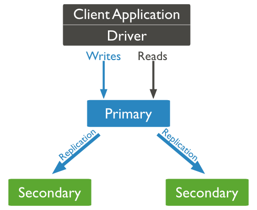
How Replication Works in MongoDB
MongoDB achieves replication by the use of replica set. A replica set is a group of mongod instances that host the same data set. In a replica, one node is primary node that receives all write operations. All other instances, such as secondaries, apply operations from the primary so that they have the same data set. * * Replica set can have only one primary node.
- Replica set is a group of two or more nodes (generally minimum 3 nodes are required).
- In a replica set, one node is primary node and remaining nodes are secondary.
- All data replicates from primary to secondary node.
- At the time of automatic failover or maintenance, election establishes for primary and a new primary node is elected.
- After the recovery of failed node, it again join the replica set and works as a secondary node.
- A typical diagram of MongoDB replication is shown in which client application always interact with the primary node and the primary node then replicates the data to the secondary nodes.
Replica Set Features
- A cluster of N nodes
- Any one node can be primary
- All write operations go to primary
- Automatic failover
- Automatic recovery
- Consensus election of primary
Set Up a Replica Set
In this tutorial, we will convert standalone MongoDB instance to a replica set. To convert to replica set, following are the steps:
- Shutdown already running MongoDB server.
- Start the MongoDB server by specifying -- replSet option. Following is the basic syntax of --replSet −
mongod --port "PORT" --dbpath "YOUR_DB_DATA_PATH" --replSet "REPLICA_SET_INSTANCE_NAME"Example
mongod --port 27017 --dbpath "D:\set up\mongodb\data" --replSet rs0- It will start a mongod instance with the name rs0, on port 27017.
- Now start the command prompt and connect to this mongod instance.
- In Mongo client, issue the command rs.initiate() to initiate a new replica set.
- To check the replica set configuration, issue the command rs.conf(). To check the status of replica set issue the command rs.status().
Add Members to Replica Set
To add members to replica set, start mongod instances on multiple machines. Now start a mongo client and issue a command rs.add().
Syntax
>rs.add(HOST_NAME:PORT)Example
Suppose your mongod instance name is mongod1.net and it is running on port 27017. To add this instance to replica set, issue the command rs.add() in Mongo client.
>rs.add("mongod1.net:27017")
>
You can add mongod instance to replica set only when you are connected to primary node. To check whether you are connected to primary or not, issue the command db.isMaster() in mongo client.
Sharding
Sharding is the process of storing data records across multiple machines and it is MongoDB's approach to meeting the demands of data growth. As the size of the data increases, a single machine may not be sufficient to store the data nor provide an acceptable read and write throughput. Sharding solves the problem with horizontal scaling. With sharding, you add more machines to support data growth and the demands of read and write operations.
Why Sharding?
- In replication, all writes go to master node
- Latency sensitive queries still go to master
- Single replica set has limitation of 12 nodes
- Memory can't be large enough when active dataset is big
- Local disk is not big enough
- Vertical scaling is too expensive
Sharding in MongoDB
The following diagram shows the sharding in MongoDB using sharded cluster.
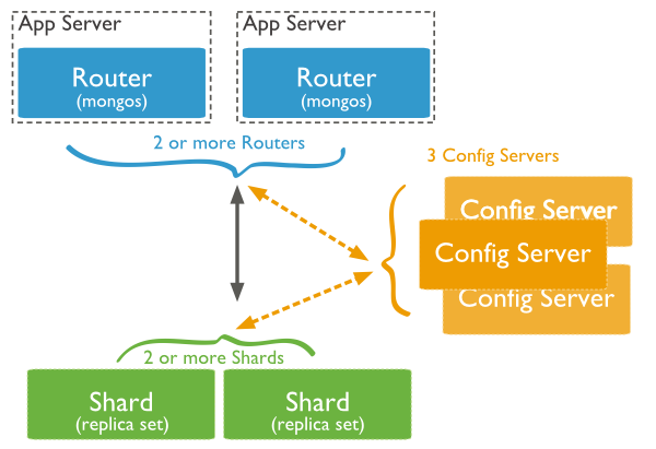
In the following diagram, there are three main components −
-
Shards − Shards are used to store data. They provide high availability and data consistency. In production environment, each shard is a separate replica set.
-
Config Servers − Config servers store the cluster's metadata. This data contains a mapping of the cluster's data set to the shards. The query router uses this metadata to target operations to specific shards. In production environment, sharded clusters have exactly 3 config servers.
-
Query Routers − Query routers are basically mongo instances, interface with client applications and direct operations to the appropriate shard. The query router processes and targets the operations to shards and then returns results to the clients. A sharded cluster can contain more than one query router to divide the client request load. A client sends requests to one query router. Generally, a sharded cluster have many query routers.
Create Backup
Dump MongoDB Data
To create backup of database in MongoDB, you should use mongodump command. This command will dump the entire data of your server into the dump directory. There are many options available by which you can limit the amount of data or create backup of your remote server.
Syntax
The basic syntax of mongodump command is as follows −
>mongodumpExample
Start your mongod server. Assuming that your mongod server is running on the localhost and port 27017, open a command prompt and go to the bin directory of your mongodb instance and type the command mongodump
Consider the mycol collection has the following data.
>mongodump| Syntax | Description | Example |
|---|---|---|
| mongodump --host HOST_NAME --port PORT_NUMBER | This commmand will backup all databases of specified mongod instance. | mongodump --host tutorialspoint.com --port 27017 |
| mongodump --dbpath DB_PATH --out BACKUP_DIRECTORY | This command will backup only specified database at specified path. | mongodump --dbpath /data/db/ --out /data/backup/ |
| mongodump --collection COLLECTION --db DB_NAME | This command will backup only specified collection of specified database. | mongodump --collection mycol --db test |
Restore data
To restore backup data MongoDB's mongorestore command is used. This command restores all of the data from the backup directory.
Syntax
The basic syntax of mongorestore command is −
>mongorestore###Deployment
Python callable()
What is a “callable” in Python?
Markdown tutorial
A quick reference and showcase for markdown
Packing and Unpacking Arguments in Python
Unpacking
Consider a function which takes 3 arguments and we have a list of size 3 with us that has all arguments for the function. If we simply pass list to the function, the call doesn’t work. It’ll give you an error as shown below.
def fun(a, b, c, d):
    print(a, b, c, d)

my_list = [1, 2, 3, 4]

fun(my_list)
Error:
TypeError: fun() missing 2 required positional arguments: 'b' and 'c'
We can use * to unpack the list so that all elements of it can be passed as different parameters.
# A sample function that takes 4 arguments
# and prints the,
def fun(a, b, c, d):
    print(a, b, c, d)

# Driver Code
my_list = [1, 2, 3, 4]

# Unpacking list into four arguments
fun(*my_list)
Output:
(1, 2, 3, 4)
Another example
# A Python program to demonstrate use
# of packing

# This function uses packing to sum
# unknown number of arguments
def mySum(*args):
    sum = 0
    for i in range(0, len(args)):
        sum = sum + args[i]
    return sum

# Driver code
print(mySum(1, 2, 3, 4, 5))
print(mySum(10, 20))
Output:
15
30
** is used for dictionaries
# A sample program to demonstrate unpacking of
# dictionary items using **
def fun(a, b, c):
    print(a, b, c)

# A call with unpacking of dictionary
d = {'a':2, 'b':4, 'c':10}
fun(**d)
--
Output:
2 4 10
Another example:
# A Python program to demonstrate packing of
# dictionary items using **
def fun(**kwargs):

    # kwargs is a dict
    print(type(kwargs))

    # Printing dictionary items
    for key in kwargs:
        print("%s = %s" % (key, kwargs[key]))

# Driver code
fun(name="geeks", ID="101", language="Python")
Output:
<class 'dict'>
language = Python
name = geeks
ID = 101
Packing:
Now, consider a situation when we don’t know how many arguments need to be passed to a python function, we can use Packing to pack all arguments in a tuple and then use it according to our convenience.
# a function that uses packing to print unknown number of arguments
def friends(*names):
    for name in names:
        print(name)

friends('Tom')
friends('Tom', 'Jerry')
Output:
Tom
Tom
Jerry
suds in python
sqlalchemy tutorial
Object relational tutorial
The SQLAlchemy Object Relational Mapper presents a method of associating user-defined Python classes with database tables, and instances of those classes (objects) with rows in their corresponding tables. It includes a system that transparently synchronizes all changes in state between objects and their related rows, called a unit of work, as well as a system for expressing database queries in terms of the user defined classes and their defined relationships between each other.
Version Check
>>> import sqlalchemy
>>> sqlalchemy.__version__
Output:
1.3.0Connecting
For postgres:
>>> from sqlalchemy import create_engine
>>> engine = create_engine('postgresql://postgres:postgres@localhost/[DBNAME]', echo=True)
The echo flag is a shortcut to setting up SQLAlchemy logging, which is accomplished via Python’s standard logging module. With it enabled, we’ll see all the generated SQL produced.
The return value of create_engine() is an instance of Engine, and it represents the core interface to the database, adapted through a dialect that handles the details of the database and DBAPI in use.
For sqlite:
>>> from sqlalchemy import create_engine
>>> engine = create_engine('sqlite:///:memory:', echo=True)
Declare a mapping
When using the ORM, the configurational process starts by describing the database tables we’ll be dealing with, and then by defining our own classes which will be mapped to those tables. In modern SQLAlchemy, these two tasks are usually performed together, using a system known as Declarative, which allows us to create classes that include directives to describe the actual database table they will be mapped to.
Classes mapped using the Declarative system are defined in terms of a base class which maintains a catalog of classes and tables relative to that base - this is known as the declarative base class. Our application will usually have just one instance of this base in a commonly imported module. We create the base class using the declarative_base() function, as follows:
>>> from sqlalchemy.ext.declarative import declarative_base
>>> Base = declarative_base()
Now that we have a “base”, we can define any number of mapped classes in terms of it. We will start with just a single table called users. A new class called User will be the class to which we map this table.
>>> from sqlalchemy import Column, Integer, String
>>> class User(Base):
...     __tablename__ = 'users'
...
...     id = Column(Integer, primary_key=True)
...     name = Column(String)
...     fullname = Column(String)
...     nickname = Column(String)
...
...     def __repr__(self):
...        return "<User(name='%s', fullname='%s', nickname='%s')>" % (
...                             self.name, self.fullname, self.nickname)
A class using Declarative at a minimum needs a tablename attribute, and at least one Column which is part of a primary key 1.
When our class is constructed, Declarative replaces all the Column objects with special Python accessors known as descriptors; this is a process known as instrumentation. The “instrumented” mapped class will provide us with the means to refer to our table in a SQL context as well as to persist and load the values of columns from the database.
object.__repr__(self)
Called by the repr() built-in function to compute the “official” string representation of an object. If at all possible, this should look like a valid Python expression that could be used to recreate an object with the same value (given an appropriate environment). If this is not possible, a string of the form <...some useful description...> should be returned. The return value must be a string object. If a class defines __repr__() but not __str__(), then __repr__() is also used when an “informal” string representation of instances of that class is required.
This is typically used for debugging, so it is important that the representation is information-rich and unambiguous.
Create a Schema
With our User class constructed via the Declarative system, we have defined information about our table, known as table metadata. The object used by SQLAlchemy to represent this information for a specific table is called the Table object, and here Declarative has made one for us. We can see this object by inspecting the table attribute:
>>> User.__table__
Table('users', MetaData(bind=None),
            Column('id', Integer(), table=<users>, primary_key=True, nullable=False),
            Column('name', String(), table=<users>),
            Column('fullname', String(), table=<users>),
            Column('nickname', String(), table=<users>), schema=None)
The Table object is a member of a larger collection known as MetaData. When using Declarative, this object is available using the .metadata attribute of our declarative base class.
The MetaData is a registry which includes the ability to emit a limited set of schema generation commands to the database.
CREATE TABLE statement
>>> Base.metadata.create_all(engine)Output:
SELECT ...
PRAGMA table_info("users")
()
CREATE TABLE users (
    id INTEGER NOT NULL, name VARCHAR,
    fullname VARCHAR,
    nickname VARCHAR,
    PRIMARY KEY (id)
)
()
COMMIT
Create an Instance of the mapped class
With mappings complete, let’s now create and inspect a User object:
>>> ed_user = User(name='ed', fullname='Ed Jones', nickname='edsnickname')
>>> ed_user.name
'ed'
>>> ed_user.nickname
'edsnickname'
>>> str(ed_user.id)
'None'
Creating a Session
We’re now ready to start talking to the database. The ORM’s “handle” to the database is the Session. When we first set up the application, at the same level as our create_engine() statement, we define a Session class which will serve as a factory for new Session objects:
>>> from sqlalchemy.orm import sessionmaker
>>> Session = sessionmaker(bind=engine)
In the case where your application does not yet have an Engine when you define your module-level objects, just set it up like this:
>>> Session = sessionmaker()Later, when you create your engine with create_engine(), connect it to the Session using configure():
>>> Session.configure(bind=engine) # once engine is availableThis custom-made Session class will create new Session objects which are bound to our database. Other transactional characteristics may be defined when calling sessionmaker as well; these are described in a later chapter. Then, whenever you need to have a conversation with the database, you instantiate a Session:
>>> session = Session()The above Session is associated with our SQLite-enabled Engine, but it hasn’t opened any connections yet. When it’s first used, it retrieves a connection from a pool of connections maintained by the Engine, and holds onto it until we commit all changes and/or close the session object.
Adding and Updating Objects
To persist our User object, we add() it to our Session:
>>> ed_user = User(name='ed', fullname='Ed Jones', nickname='edsnickname')
>>> session.add(ed_user)
t this point, we say that the instance is pending; no SQL has yet been issued and the object is not yet represented by a row in the database. The Session will issue the SQL to persist Ed Jones as soon as is needed, using a process known as a flush. If we query the database for Ed Jones, all pending information will first be flushed, and the query is issued immediately thereafter.
For example, below we create a new Query object which loads instances of User. We “filter by” the name attribute of ed, and indicate that we’d like only the first result in the full list of rows. A User instance is returned which is equivalent to that which we’ve added:
SQL>>> our_user = session.query(User).filter_by(name='ed').first()
>>> our_user
<User(name='ed', fullname='Ed Jones', nickname='edsnickname')>
In fact, the Session has identified that the row returned is the same row as one already represented within its internal map of objects, so we actually got back the identical instance as that which we just added:
>>> ed_user is our_user
True
We can add more User objects at once using add_all():
>>> session.add_all([
...     User(name='wendy', fullname='Wendy Williams', nickname='windy'),
...     User(name='mary', fullname='Mary Contrary', nickname='mary'),
...     User(name='fred', fullname='Fred Flintstone', nickname='freddy')])
Also, we’ve decided Ed’s nickname isn’t that great, so lets change it:
>>> ed_user.nickname = 'eddie'The Session is paying attention. It knows, for example, that Ed Jones has been modified:
>>> session.dirtyIdentitySet([<User(name='ed', fullname='Ed Jones', nickname='eddie')>])
and that three new User objects are pending:
>>> session.new
IdentitySet([<User(name='wendy', fullname='Wendy Williams', nickname='windy')>,
<User(name='mary', fullname='Mary Contrary', nickname='mary')>,
<User(name='fred', fullname='Fred Flintstone', nickname='freddy')>])
We tell the Session that we’d like to issue all remaining changes to the database and commit the transaction, which has been in progress throughout. We do this via commit(). The Session emits the UPDATE statement for the nickname change on “ed”, as well as INSERT statements for the three new User objects we’ve added:
SQL>>> session.commit()commit() flushes the remaining changes to the database, and commits the transaction. The connection resources referenced by the session are now returned to the connection pool. Subsequent operations with this session will occur in a new transaction, which will again re-acquire connection resources when first needed.
After the Session inserts new rows in the database, all newly generated identifiers and database-generated defaults become available on the instance, either immediately or via load-on-first-access. In this case, the entire row was re-loaded on access because a new transaction was begun after we issued commit(). SQLAlchemy by default refreshes data from a previous transaction the first time it’s accessed within a new transaction, so that the most recent state is available. The level of reloading is configurable as is described in Using the Session.
Rolling Back
Since the Session works within a transaction, we can roll back changes made too. Let’s make two changes that we’ll revert; ed_user’s user name gets set to Edwardo:
>>> ed_user.name = 'Edwardo'and we’ll add another erroneous user, fake_user:
>>> fake_user = User(name='fakeuser', fullname='Invalid', nickname='12345')
>>> session.add(fake_user)
Querying the session, we can see that they’re flushed into the current transaction:
SQL>>> session.query(User).filter(User.name.in_(['Edwardo', 'fakeuser'])).all()
[<User(name='Edwardo', fullname='Ed Jones', nickname='eddie')>, <User(name='fakeuser', fullname='Invalid', nickname='12345')>]
issuing a SELECT illustrates the changes made to the database:
SQL>>> session.query(User).filter(User.name.in_(['ed', 'fakeuser'])).all()
[<User(name='ed', fullname='Ed Jones', nickname='eddie')>]
Querying
A Query object is created using the query() method on Session. This function takes a variable number of arguments, which can be any combination of classes and class-instrumented descriptors. Below, we indicate a Query which loads User instances. When evaluated in an iterative context, the list of User objects present is returned:
SQL>>> for instance in session.query(User).order_by(User.id):
...     print(instance.name, instance.fullname)
ed Ed Jones
wendy Wendy Williams
mary Mary Contrary
fred Fred Flintstone
The Query also accepts ORM-instrumented descriptors as arguments. Any time multiple class entities or column-based entities are expressed as arguments to the query() function, the return result is expressed as tuples:
>>> for name, fullname in session.query(User.name, User.fullname):
...     print(name, fullname)
ed Ed Jones
wendy Wendy Williams
mary Mary Contrary
fred Fred Flintstone
The tuples returned by Query are named tuples, supplied by the KeyedTuple class, and can be treated much like an ordinary Python object. The names are the same as the attribute’s name for an attribute, and the class name for a class:
SQL>>> for row in session.query(User, User.name).all():
...    print(row.User, row.name)
<User(name='ed', fullname='Ed Jones', nickname='eddie')> ed
<User(name='wendy', fullname='Wendy Williams', nickname='windy')> wendy
<User(name='mary', fullname='Mary Contrary', nickname='mary')> mary
<User(name='fred', fullname='Fred Flintstone', nickname='freddy')> fred
You can control the names of individual column expressions using the label() construct, which is available from any ColumnElement-derived object, as well as any class attribute which is mapped to one (such as User.name):
SQL>>> for row in session.query(User.name.label('name_label')).all():
...    print(row.name_label)
ed
wendy
mary
fred
Basic Relationship Patterns
The imports used for each of the following sections is as follows:
from sqlalchemy import Table, Column, Integer, ForeignKey
from sqlalchemy.orm import relationship
from sqlalchemy.ext.declarative import declarative_base

Base = declarative_base()
One To Many
A one to many relationship places a foreign key on the child table referencing the parent. relationship() is then specified on the parent, as referencing a collection of items represented by the child:
class Parent(Base):
    __tablename__ = 'parent'
    id = Column(Integer, primary_key=True)
    children = relationship("Child")

class Child(Base):
    __tablename__ = 'child'
    id = Column(Integer, primary_key=True)
    parent_id = Column(Integer, ForeignKey('parent.id'))
To establish a bidirectional relationship in one-to-many, where the “reverse” side is a many to one, specify an additional relationship() and connect the two using the relationship.back_populates parameter:
class Parent(Base):
    __tablename__ = 'parent'
    id = Column(Integer, primary_key=True)
    children = relationship("Child", back_populates="parent")

class Child(Base):
    __tablename__ = 'child'
    id = Column(Integer, primary_key=True)
    parent_id = Column(Integer, ForeignKey('parent.id'))
    parent = relationship("Parent", back_populates="children")
Child will get a parent attribute with many-to-one semantics.
Alternatively, the backref option may be used on a single relationship() instead of using back_populates:
class Parent(Base):
    __tablename__ = 'parent'
    id = Column(Integer, primary_key=True)
    children = relationship("Child", backref="parent")
Many To One
Many to one places a foreign key in the parent table referencing the child. relationship() is declared on the parent, where a new scalar-holding attribute will be created:
class Parent(Base):
    __tablename__ = 'parent'
    id = Column(Integer, primary_key=True)
    child_id = Column(Integer, ForeignKey('child.id'))
    child = relationship("Child")

class Child(Base):
    __tablename__ = 'child'
    id = Column(Integer, primary_key=True)
Bidirectional behavior is achieved by adding a second relationship() and applying the relationship.back_populates parameter in both directions:
class Parent(Base):
    __tablename__ = 'parent'
    id = Column(Integer, primary_key=True)
    child_id = Column(Integer, ForeignKey('child.id'))
    child = relationship("Child", back_populates="parents")

class Child(Base):
    __tablename__ = 'child'
    id = Column(Integer, primary_key=True)
    parents = relationship("Parent", back_populates="child")
Alternatively, the backref parameter may be applied to a single relationship(), such as Parent.child:
class Parent(Base):
    __tablename__ = 'parent'
    id = Column(Integer, primary_key=True)
    child_id = Column(Integer, ForeignKey('child.id'))
    child = relationship("Child", backref="parents")
One To One
One To One is essentially a bidirectional relationship with a scalar attribute on both sides. To achieve this, the uselist flag indicates the placement of a scalar attribute instead of a collection on the “many” side of the relationship. To convert one-to-many into one-to-one:
class Parent(Base):
    __tablename__ = 'parent'
    id = Column(Integer, primary_key=True)
    child = relationship("Child", uselist=False, back_populates="parent")

class Child(Base):
    __tablename__ = 'child'
    id = Column(Integer, primary_key=True)
    parent_id = Column(Integer, ForeignKey('parent.id'))
    parent = relationship("Parent", back_populates="child")
Or for many-to-one:
class Parent(Base):
    __tablename__ = 'parent'
    id = Column(Integer, primary_key=True)
    child_id = Column(Integer, ForeignKey('child.id'))
    child = relationship("Child", back_populates="parent")

class Child(Base):
    __tablename__ = 'child'
    id = Column(Integer, primary_key=True)
    parent = relationship("Parent", back_populates="child", uselist=False)
As always, the relationship.backref and backref() functions may be used in lieu of the relationship.back_populates approach; to specify uselist on a backref, use the backref() function:
from sqlalchemy.orm import backref

class Parent(Base):
    __tablename__ = 'parent'
    id = Column(Integer, primary_key=True)
    child_id = Column(Integer, ForeignKey('child.id'))
    child = relationship("Child", backref=backref("parent", uselist=False))
Many To Many
Many to Many adds an association table between two classes. The association table is indicated by the secondary argument to relationship(). Usually, the Table uses the MetaData object associated with the declarative base class, so that the ForeignKey directives can locate the remote tables with which to link:
association_table = Table('association', Base.metadata,
    Column('left_id', Integer, ForeignKey('left.id')),
    Column('right_id', Integer, ForeignKey('right.id'))
)

class Parent(Base):
    __tablename__ = 'left'
    id = Column(Integer, primary_key=True)
    children = relationship("Child",
                    secondary=association_table)

class Child(Base):
    __tablename__ = 'right'
    id = Column(Integer, primary_key=True)
For a bidirectional relationship, both sides of the relationship contain a collection. Specify using relationship.back_populates, and for each relationship() specify the common association table:
association_table = Table('association', Base.metadata,
    Column('left_id', Integer, ForeignKey('left.id')),
    Column('right_id', Integer, ForeignKey('right.id'))
)

class Parent(Base):
    __tablename__ = 'left'
    id = Column(Integer, primary_key=True)
    children = relationship(
        "Child",
        secondary=association_table,
        back_populates="parents")

class Child(Base):
    __tablename__ = 'right'
    id = Column(Integer, primary_key=True)
    parents = relationship(
        "Parent",
        secondary=association_table,
        back_populates="children")
When using the backref parameter instead of relationship.back_populates, the backref will automatically use the same secondary argument for the reverse relationship:
association_table = Table('association', Base.metadata,
    Column('left_id', Integer, ForeignKey('left.id')),
    Column('right_id', Integer, ForeignKey('right.id'))
)

class Parent(Base):
    __tablename__ = 'left'
    id = Column(Integer, primary_key=True)
    children = relationship("Child",
                    secondary=association_table,
                    backref="parents")

class Child(Base):
    __tablename__ = 'right'
    id = Column(Integer, primary_key=True)
The secondary argument of relationship() also accepts a callable that returns the ultimate argument, which is evaluated only when mappers are first used. Using this, we can define the association_table at a later point, as long as it’s available to the callable after all module initialization is complete:
class Parent(Base):
    __tablename__ = 'left'
    id = Column(Integer, primary_key=True)
    children = relationship("Child",
                    secondary=lambda: association_table,
                    backref="parents")
With the declarative extension in use, the traditional “string name of the table” is accepted as well, matching the name of the table as stored in Base.metadata.tables:

class Parent(Base):
    __tablename__ = 'left'
    id = Column(Integer, primary_key=True)
    children = relationship("Child",
                    secondary="association",
                    backref="parents")
pickle library in python
Iterators and generators in python
How to create iterations easily using python generators, how is it different from iterators and normal functions, and why you should use it.
Python Web Server Gateway Interface (WSGI)
Introduction
WSGI is not a server, a python module, a framework, an API or any kind of software. It is just an interface specification by which server and application communicate. Both server and application interface sides are specified in the PEP 3333. If an application (or framework or toolkit) is written to the WSGI spec then it will run on any server written to that spec.
WSGI applications (meaning WSGI compliant) can be stacked. Those in the middle of the stack are called middleware and must implement both sides of the WSGI interface, application and server. For the application in top of it it will behave as a server and for the application (or server) bellow as an application.
A WSGI server (meaning WSGI compliant) only receives the request from the client, pass it to the application and then send the response returned by the application to the client. It does nothing else. All the gory details must be supplied by the application or middleware.
Summary of Specification
The PEP specifies three roles: the role of a server, the role of a framework/app, and the role of a middleware object.
Web server side
The server must provide two things: an environ dictionary, and a start_response function. The environ dictionary needs to have the usual things present -- it's similar to the CGI environment. start_response is a callable that takes two arguments, status -- containing a standard HTTP status string like 200 OK -- and response_headers -- a list of standard HTTP response headers.
The Web server dispatches a request to the framework/app by calling the application:
iterable = app(environ, start_response)
for data in iterable:
   # send data to client
It's the framework/app's responsibility to build the headers, call start_response, and build the data returned in iterable. It's the Web server's responsibility to serve both the headers and the data up via HTTP.
Web framework/app side
The Web framework/app is represented to the server as a Python callable. It can be a class, an object, or a function. The arguments to init, call, or the function must be as above: an environ object and a start_response callable.
The Web framework/app must call start_response before returning or yielding any data.
The Web framework/app should return any data in an iterable form -- e.g. return [ page ].
Middleware
Middleware components must obey both the Web server side and the Web app/framework side of things, plus a few more minor niggling restrictions. Middleware should be as transparent as possible.
An example WSGI application
Here's a very simple WSGI application that returns a static "Hello world!" page.
def simple_app(environ, start_response):
    status = '200 OK'
    response_headers = [('Content-type','text/plain')]
    start_response(status, response_headers)
    return ['Hello world!\n']
Here's a very simple middleware application that uppercases everything sent:
class Upperware:
   def __init__(self, app):
      self.wrapped_app = app

   def __call__(self, environ, start_response):
      for data in self.wrapped_app(environ, start_response):
         return data.upper()
To instantiate/run these from the server's perspective, you just do the obvious:
serve(simple_app)
or
wrapped_app = Upperware(simple_app)
serve(wrapped_app)
Yes, it can be that simple: here's my code for running Trac via scgiserver.
#!/usr/bin/env python
from trac.web.main import dispatch_request as app
from scgiserver import serve_application

PREFIX=''
PORT=4101

serve_application(app, PREFIX, PORT)
Python functions
Functions in Python that covers how to write functions, how to call them, and more!
Recommend Projects
-
 React
React
A declarative, efficient, and flexible JavaScript library for building user interfaces.
-
Vue.js
🖖 Vue.js is a progressive, incrementally-adoptable JavaScript framework for building UI on the web.
-
 Typescript
TypeScript is a superset of JavaScript that compiles to clean JavaScript output.
-
TensorFlow
An Open Source Machine Learning Framework for Everyone
-
Django
The Web framework for perfectionists with deadlines.
-
 Laravel
A PHP framework for web artisans
-
D3
Bring data to life with SVG, Canvas and HTML. 📊📈🎉
-
Recommend Topics
-
javascript
JavaScript (JS) is a lightweight interpreted programming language with first-class functions.
-
web
Some thing interesting about web. New door for the world.
-
server
A server is a program made to process requests and deliver data to clients.
-
Machine learning
Machine learning is a way of modeling and interpreting data that allows a piece of software to respond intelligently.
-
Visualization
Some thing interesting about visualization, use data art
-
Game
Some thing interesting about game, make everyone happy.
Recommend Org
-
Facebook
We are working to build community through open source technology. NB: members must have two-factor auth.
-
Microsoft
Open source projects and samples from Microsoft.
-
Google
Google ❤️ Open Source for everyone.
-
Alibaba
Alibaba Open Source for everyone
-
D3
Data-Driven Documents codes.
-
Tencent
China tencent open source team.