The goals / steps of this project are the following:
- Compute the camera calibration matrix and distortion coefficients given a set of chessboard images.
- Apply a distortion correction to raw images.
- Use color transforms, gradients, etc., to create a thresholded binary image.
- Apply a perspective transform to rectify binary image ("birds-eye view").
- Detect lane pixels and fit to find the lane boundary.
- Determine the curvature of the lane and vehicle position with respect to center.
- Warp the detected lane boundaries back onto the original image.
- Output visual display of the lane boundaries and numerical estimation of lane curvature and vehicle position.
The code for this step is contained in the first code cell of the IPython notebook located in "./examples/camera_calibration.ipynb"
I start by preparing "object points", which will be the (x, y, z) coordinates of the chessboard corners in the world. Here I am assuming the chessboard is fixed on the (x, y) plane at z=0, such that the object points are the same for each calibration image. Thus, objp is just a replicated array of coordinates, and objpoints will be appended with a copy of it every time I successfully detect all chessboard corners in a test image. imgpoints will be appended with the (x, y) pixel position of each of the corners in the image plane with each successful chessboard detection.
I then used the output objpoints and imgpoints to compute the camera calibration and distortion coefficients using the cv2.calibrateCamera() function. I applied this distortion correction to the test image using the cv2.undistort() function and obtained this result:
A few images were not suitable for calibration because not all inner corners were visible.

I appled the distortion correction to the test images test1.jpg
- Load mtx and dist from pickle file that I have stored during camera calibration (previous step)
- Undistort this image
See below for the result

To find the best combination of:
- color space
- color channel
- gradient method's (none, sobel x, sobel y, sobel magnitude or sobel gradient) -> 1 or a combination
- min. and max. threshold per method I have made a script to calculate all possible combinations of previous parameters.
To limit the computere calculation time, I have limited myself to the following:
- HLS colorspace
- S channel
- max.combination of 2 gradient method's
- the best single performing min. and max. threshold's
The best performing combination was:
- HLS colorspace with S channel with R channel of RGB
- sobel x gradient
- kernel size 3
- min. threshold 20
- max. threshold between 135 and 255 (all more or less equal)
An example is show below:

The code for my perspective transform includes functions called:
unwarp_expand_top()
warp_shrink_top()
(file parse_video.py, lines 127-159)
The parameters are hardcodes programmed in
get_perspective_parameters()
    DST_MARGIN_X = 100

    TOP_Y = 450
    LEFT_TOP_X = 593
    RIGHT_TOP_X = 690

    BOTTOM_Y = 675
    LEFT_BOTTOM_X = 270
    RIGHT_BOTTOM_X = 1038

    src = np.float32([[LEFT_BOTTOM_X, BOTTOM_Y], [LEFT_TOP_X, TOP_Y],
                      [RIGHT_BOTTOM_X, BOTTOM_Y], [RIGHT_TOP_X, TOP_Y]])
    dst = np.float32([[LEFT_BOTTOM_X + DST_MARGIN_X, 720], [LEFT_BOTTOM_X + DST_MARGIN_X, 0],
                      [RIGHT_BOTTOM_X - DST_MARGIN_X, 720], [RIGHT_BOTTOM_X - DST_MARGIN_X, 0]])
I verified that my perspective transform was working as expected by drawing the src and dst points onto a test image and its warped counterpart to verify that the lines appear parallel in the warped image.


As as starting point I have used the 'Sliding windows' method as described in section 33 of lesson 15. This method exists of:
- Take a histogram of the lower half of the window
- Find the peak of the left and the right half of the image -> these are the starting points
- Only for training purposes: Check if the starting points are valid
- Split the image in 9 vertical windows
- For each window (starting at the bottom, working upwards), take all the points and take the mean of the pixels in that windows
- From the resulting pixels, calculate the polynomial
- Only for training purposes: Check if the curve is left, straight or right and compare it with the expected corner
- For the derived polynomial: construct a line by calculating the x for each y
The above strategy is implemented in the class FindLines (file FindLines.py), method calculate
See below for an example.

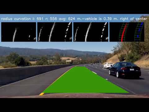
5. Calculation the radius of curvature of the lane and the position of the vehicle with respect to center.
I did this in lines 189 through 234 in my code in FindLines.py
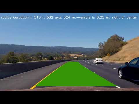
I implemented this step in lines 163 through 182 in my code in FindLines.py in the method draw_lines(). Here is an example of my result on a test image:

Click on the YouTube video below to see the intermediate steps:
Here's a link to my video result
Or click on the YouTube video below:
I have spend most time (and far too much) in finding the right gradient that was working for all the 8 test images. I didn't want to do this manual so I created an algorithm that could automatically find the best combination of threshold for the different gradient sobel method. But at the end this took too much time and was not optimal yet, so took the best solution I had so far. This is done in the files pipeline.py and pipeline_all.py
The following improvements could be done:
- Improve the algorithm to find the best gradient method OR
- Use a deep learning approach to find the polynomial
- The sliding windows method could be improved


