The fieldimager.extra from jenniferlopes

FIELDimageR.Extra: An package with new tools to support FIELDimageR software on evaluating GIS images from agriculture field trials using R.

This package was developed by Popat Pawar and Filipe Matias to help FIELDimageR users with new functions to analyze orthomosaic images from research fields. Cropping and rotating images are not necessary anymore, and there are amazing zoom capabilities provided by newly released GIS R packages. Come along with us and try this tutorial out ... We hope it helps with your research!

Resources

Installation

Step 1. How to start?

Step 2. Loading mosaics and visualizing

Step 3. Building the plot shapefile (Zoom)

Step 4. Editing the plot shapefile (Zoom)

Step 5. Building vegetation indices

Step 6. Image segmentation based on unsupervised (K-means) and supervised (Random Forest) methods to remove the soil effect

Step 7. Extracting data from field images

Step 8. Vizualizing extracted data

Step 9. Saving output files and opening them in the QGIS

Step 10. Cropping individual plots and saving

Contact

Installation

First of all, install R and RStudio. Then, in order to install R/FIELDimageR.Extra from GitHub GitHub repository, you need to install the following packages in R. For Windows users who have an R version higher than 4.0, you need to install RTools, tutorial RTools For Windows.

Now install R/FIELDimageR.Extra using the install_github function from devtools package. If necessary, use the argument type="source".

install.packages("devtools")
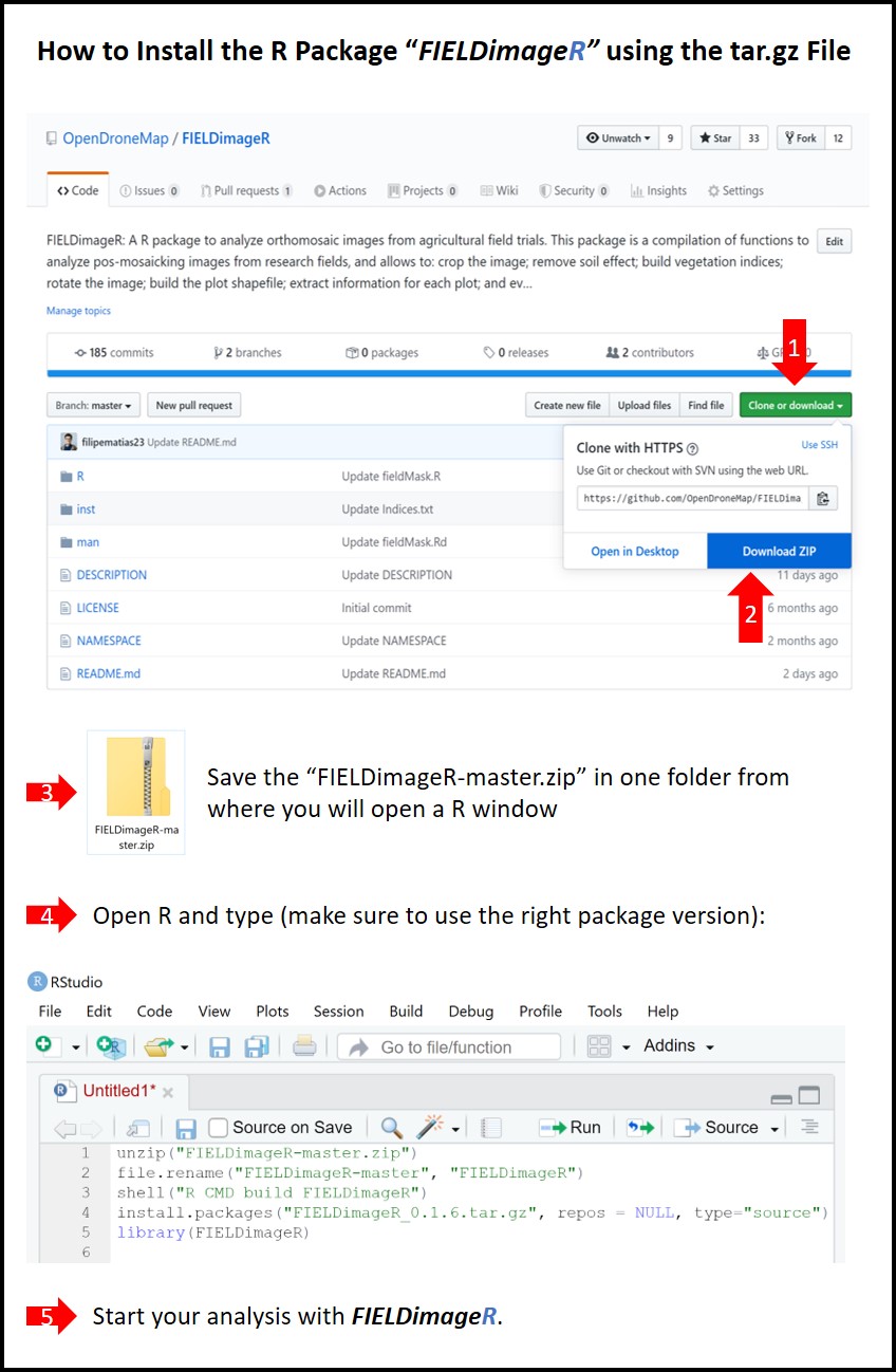
devtools::install_github("filipematias23/FIELDimageR.Extra")

If the method above doesn't work, use the next lines by downloading the FIELDimageR-master.zip file

setwd("~/FIELDimageR.Extra-main.zip") # ~ is the path from where you saved the file.zip
unzip("FIELDimageR.Extra-main.zip") 
file.rename("FIELDimageR.Extra-main", "FIELDimageR.Extra") 
shell("R CMD build FIELDimageR.Extra") # or system("R CMD build FIELDimageR.Extra")
install.packages("FIELDimageR.Extra_0.0.1.tar.gz", repos = NULL, type="source") # Make sure to use the right version (e.g. 0.0.1)

The image below from R/FIELDimageR is highlighting how to do the steps described above and install R/FIELDimageR.Extra using source code.

Using R/FIELDimageR.Extra

1. First steps

Reading necessary packages:

# Install:
install.packages(c('terra','mapview','sf','stars'))
devtools::install_github("OpenDroneMap/FIELDimageR")

# Packages:
library(FIELDimageR)
library(FIELDimageR.Extra)
library(terra)
library(mapview)
library(sf)
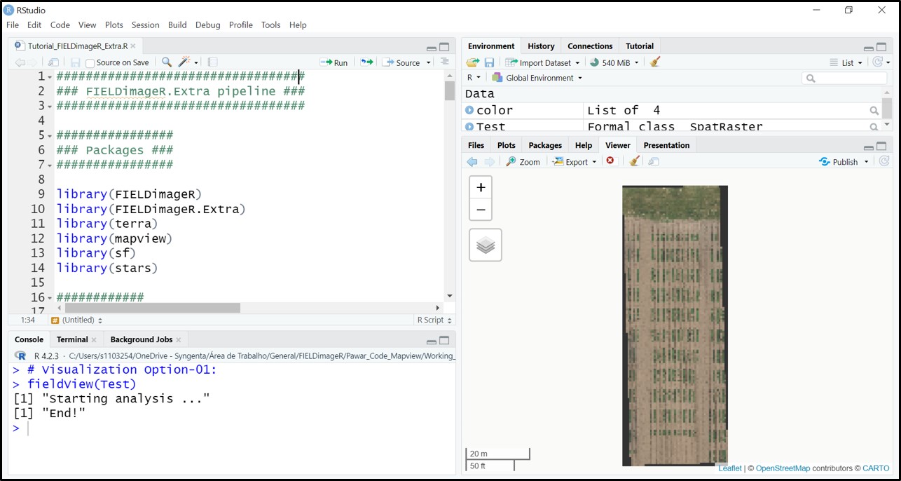
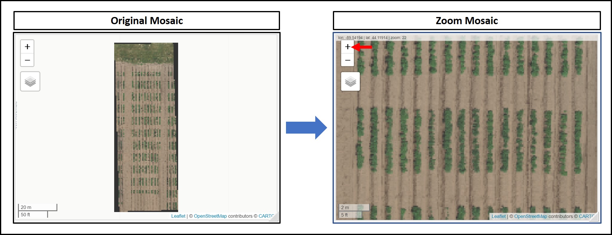
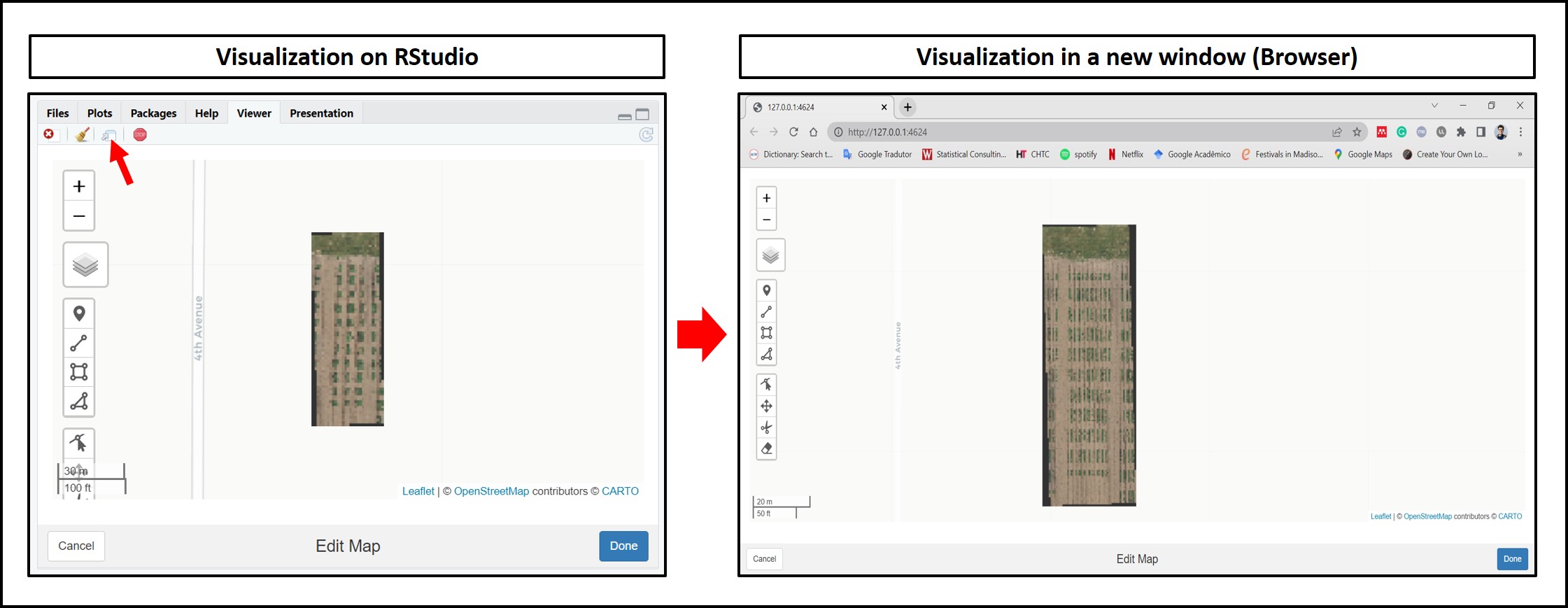
library(stars)

2. Loading mosaics and visualizing

The following example uses an image available to download here: EX1_RGB.tif. The first R/FIELDimageR.Extra function is fieldView used to visualize GIS images and grid shapefiles and zoom it out.

# Uploading an example mosaic
Test <- rast("EX1_RGB.tif")

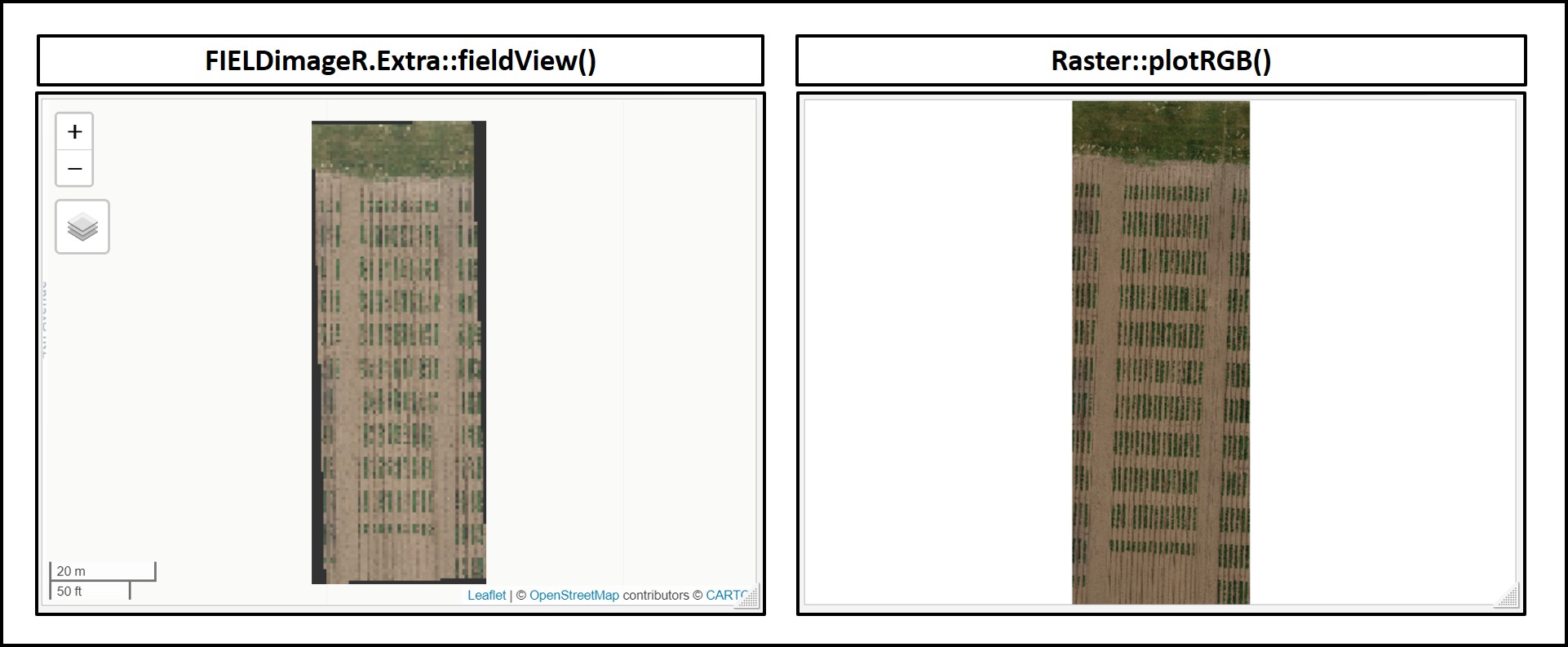
# Visualization Option-01 (FIELDimageR.Extra):
fieldView(Test)

# Visualization Option-02 (raster):
plotRGB(Test)

3. Building the plot shapefile (Zoom)

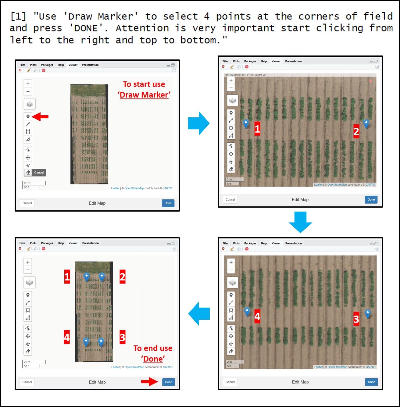
FIELDimageR.Extra allows drawing the plot shape file using the function fieldShape_render. Different from FIELDimageR::fieldShape this new function does not request straight fields and the experimental trial can be used in any direction according to the original GIS position. It is very important to highlight that four points need to be set at the corners of the trial according to the following sequence (1st point) left superior corner, (2nd point) right superior corner, (3rd point) right inferior corner, and (4th point) left inferior corner. The mosaic will be presented for visualization with the North part on the superior part (top) and the south in )the inferior part (bottom). The number of columns and rows must be informed. At this point, the experimental borders can be eliminated (check the example below.

plotShape<-fieldShape_render(mosaic = Test,
                             ncols=14,
                             nrows=9)

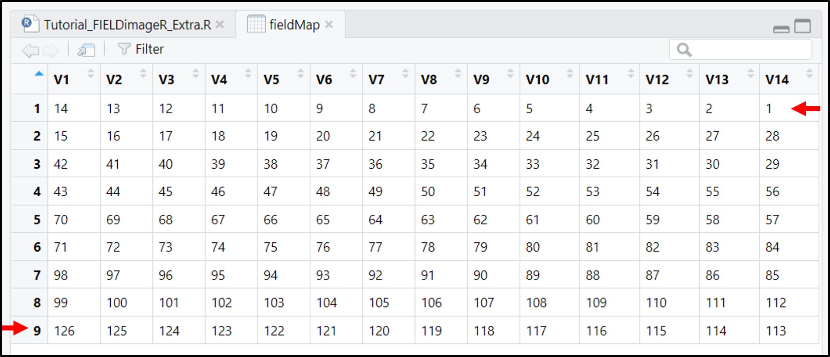
Attention: The plots are identified in ascending order from left to right and bottom to top (this is another difference from the FIELDimageR::fieldShape ) being evenly spaced and distributed inside the selected area independent of alleys.

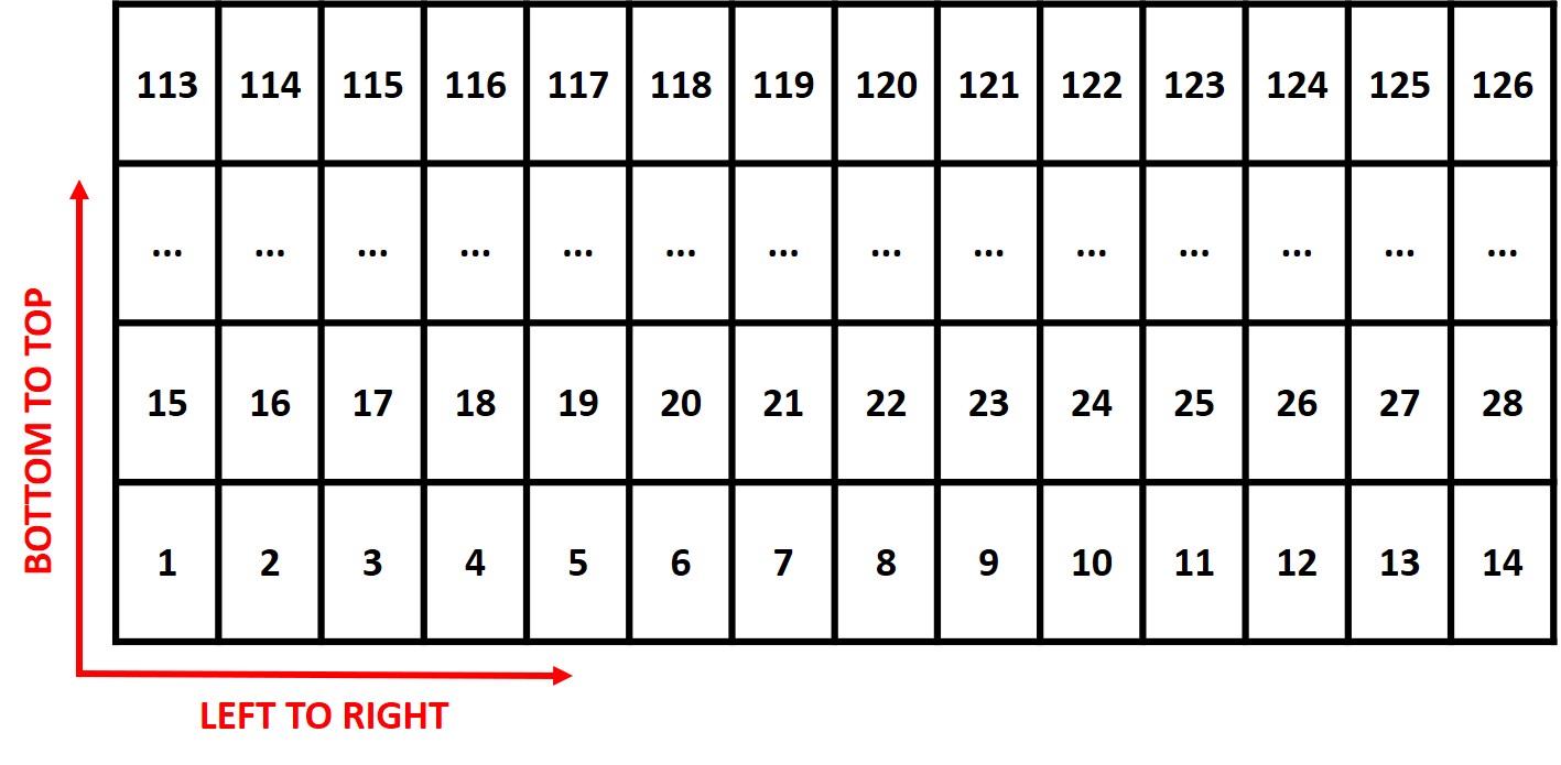
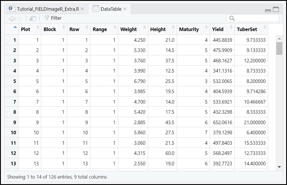
One matrix can be used to identify the plots position according to the image above. The function FIELDimageR::fieldMap can be used to specify the plot ID automatic or any other matrix (manually built) also can be used. For instance, the new column PlotID will be the new identification. You can download an external table example here: DataTable.csv.

# Reading DataTable.csv
DataTable<-read.csv("DataTable.csv",header = T)
DataTable

### Field map identification (name for each Plot). 'fieldPlot' argument can be a number or name.

fieldMap<-fieldMap(fieldPlot=DataTable$Plot, fieldColumn=DataTable$Row, fieldRow=DataTable$Range, decreasing=T)
fieldMap

# The new column PlotID is identifying the plots:
plotShape<-fieldShape_render(mosaic = Test,
                             ncols=14,
                             nrows=9,
                             fieldMap = fieldMap,
                             buffer = -0.05)

### Joing all information from 'fieldData' in one "fieldShape" file using the column 'Plot' as reference:

plotShape<-fieldShape_render(mosaic = Test,
                             ncols=14,
                             nrows=9,
                             fieldData = DataTable,
                             fieldMap = fieldMap,
                             PlotID = "Plot",
                             buffer = -0.05)
                      
# The new column PlotID is identifying the plots:                      
plotShape

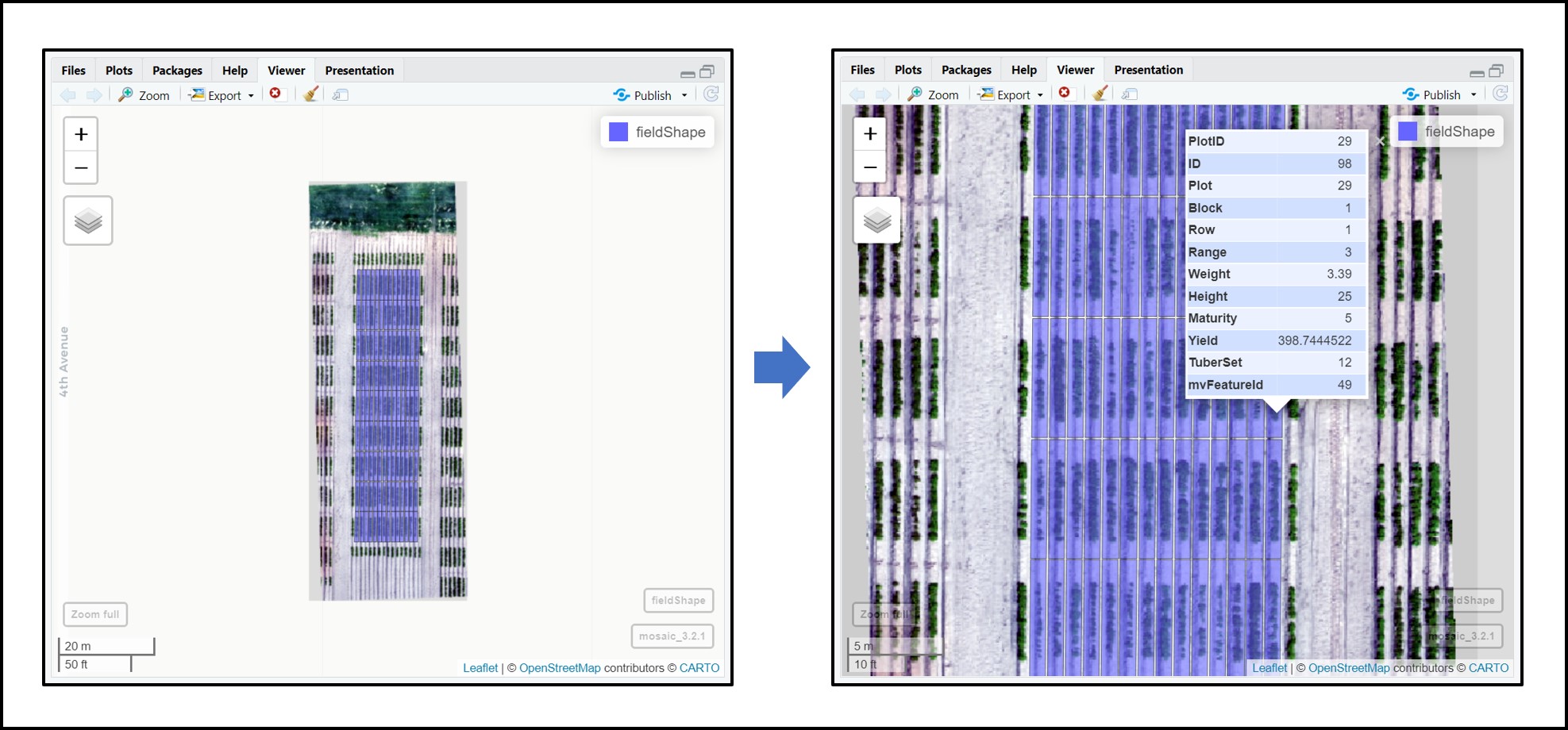
# Vizualizing new plot grid shape object with field data:
fieldView(mosaic = Test,
          fieldShape = plotShape,
          type = 2,
          alpha = 0.2)

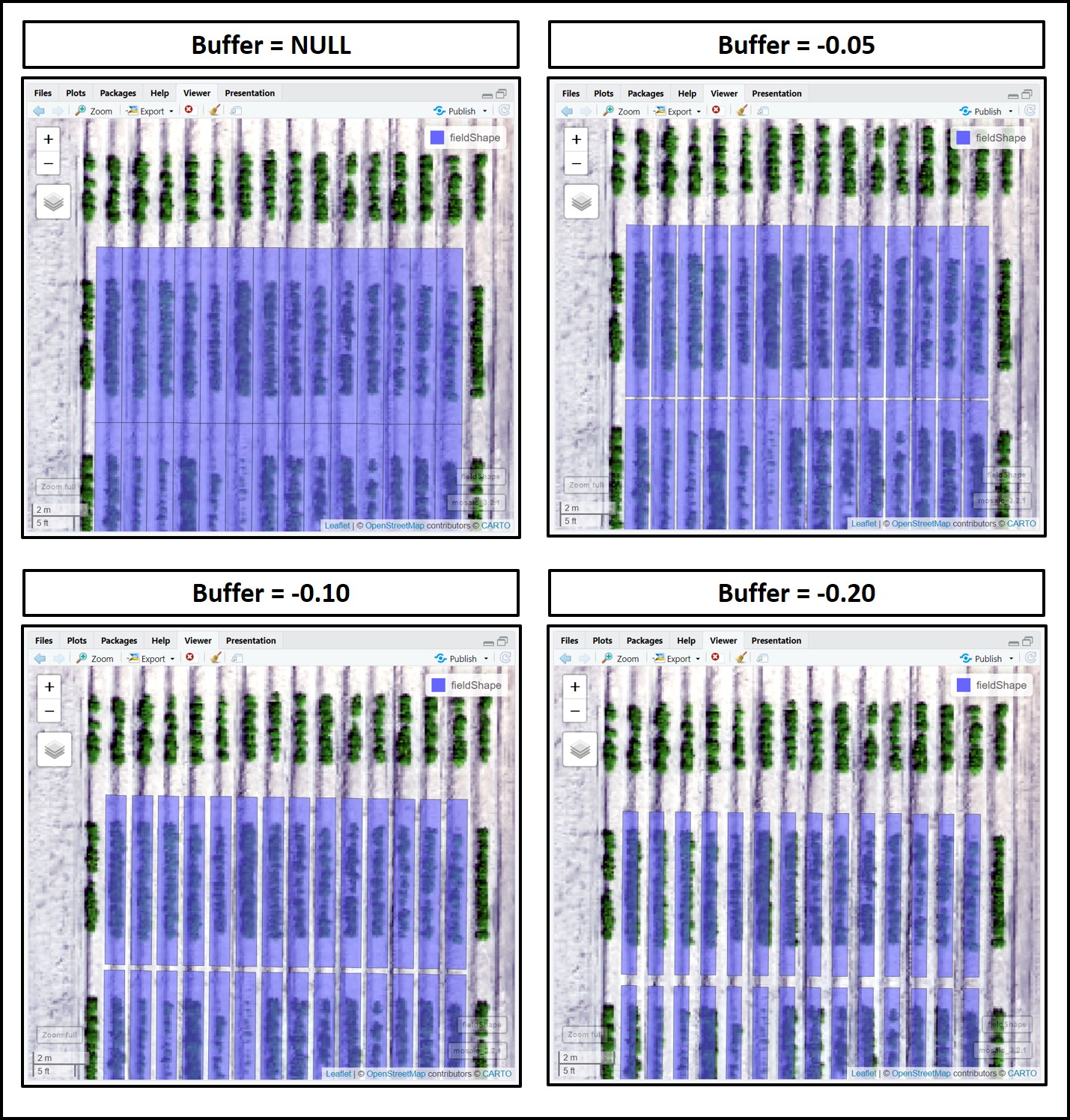
### Different plot dimensions using "Buffer":

# Buffer = NULL
Buffer.1<-fieldShape_render(mosaic = Test,
                             ncols=14,
                             nrows=9)
fieldView(mosaic = Test,
          fieldShape = Buffer.1,
          type = 2,
          alpha = 0.2)

# Buffer = -0.05
Buffer.2<-fieldShape_render(mosaic = Test,
                             ncols=14,
                             nrows=9,
                             buffer = -0.05)
fieldView(mosaic = Test,
          fieldShape = Buffer.2,
          type = 2,
          alpha = 0.2)

# Buffer = -0.10
Buffer.3<-fieldShape_render(mosaic = Test,
                             ncols=14,
                             nrows=9,
                             buffer = -0.10)
fieldView(mosaic = Test,
          fieldShape = Buffer.3,
          type = 2,
          alpha = 0.2)

# Buffer = -0.20
Buffer.4<-fieldShape_render(mosaic = Test,
                             ncols=14,
                             nrows=9,
                             buffer = -0.20)
fieldView(mosaic = Test,
          fieldShape = Buffer.4,
          type = 2,
          alpha = 0.2)

4. Editing plot shapefile (Zoom)

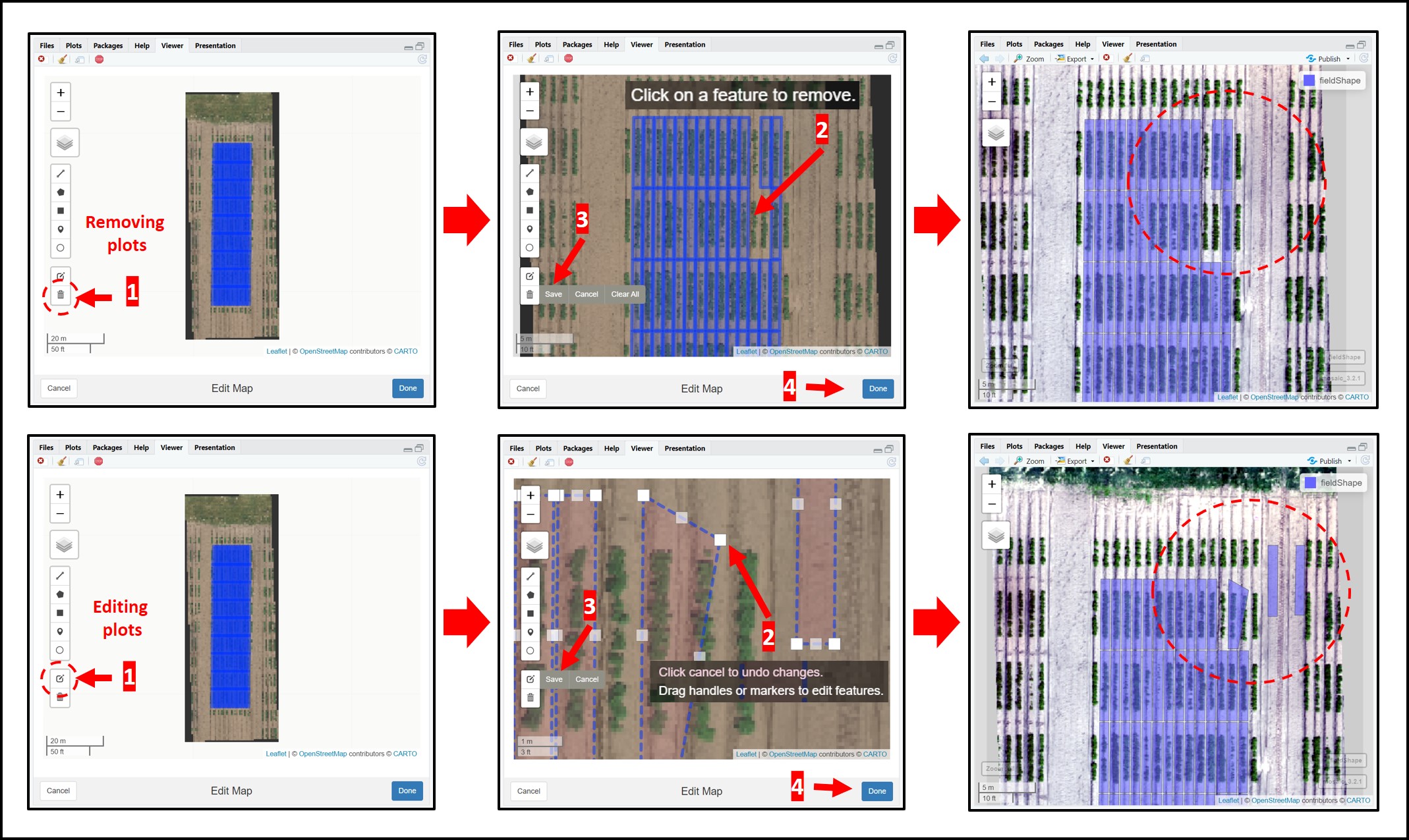
Editing, moving, deleting, and changing single plot grids in fieldShape objects is now possible with the function fieldShape_edit. Follow the image bellow to understand how this function works. Attention: do not forget to press SAVE before clicking on DONE.

# Editing plot grid shapefile:
editShape<- fieldShape_edit(mosaic=Test,
                            fieldShape=plotShape)

# Checking the edited plot grid shapefile:
fieldView(mosaic = Test,
          fieldShape = editShape,
          type = 2,
          alpha = 0.2)

5. Building vegetation indices

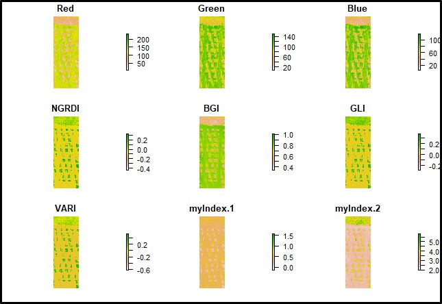
Vegetation indices still being calculated using the function FIELDimageR::fieldIndex from FIELDimageR package.

# Vegetation indices:
Test.Indices<- fieldIndex(mosaic = Test, 
                          Red = 1, Green = 2, Blue = 3, 
                          index = c("NGRDI","BGI", "GLI","VARI"), 
                          myIndex = c("(Red-Blue)/Green","2*Green/Blue"))

# To visualize single band layer:
single_layer<-Test.Indices$GLI
fieldView(single_layer,
          fieldShape = editShape,
          type = 2,
          alpha_grid = 0.2)

fieldView(single_layer,
          fieldShape = editShape,
          plotCol = c("Yield"),
          colorOptions = 'RdYlGn',
          type = 1,
          alpha_grid = 0.8)

6. Removing the soil effect

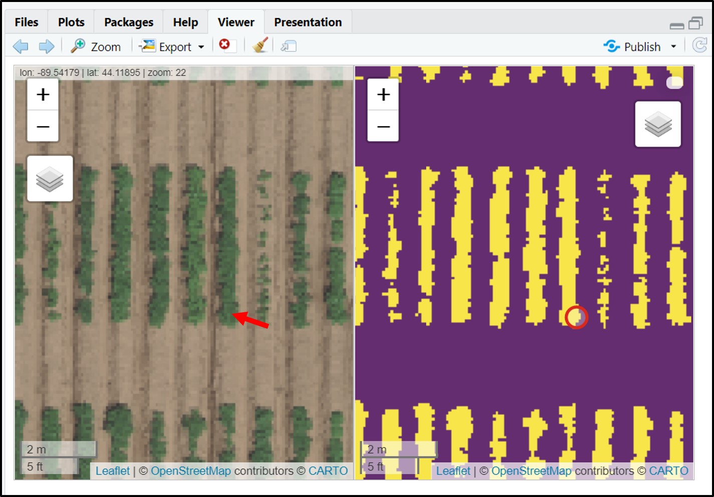
FIELDimageR.Extra introduce the function fieldKmeans as the first option to remove soil (Option_01). Based on the K-means unsupervised method. This function clusters pixels on the number of clusters decided by the user. Each cluster can be associated with plants, soil, shadows, etc. Attention: Each image/mosaic will have different cluster numbers representing plants or soil. In this example, cluster_01 is plants and cluster_02 is soil.

# Option_01 = Using fieldKmeans() to extract soil
Test.kmean<-fieldKmeans(mosaic=Test.Indices$GLI,
                   clusters = 2)
fieldView(Test.kmean)

# Check which cluster is related to plants or soil based on the color. In this example cluster 1 represents plants and cluster 2 represents soil
library(leafsync)
rgb<-fieldView(Test)
plants<-fieldView(Test.kmean==1)
sync(rgb,plants)

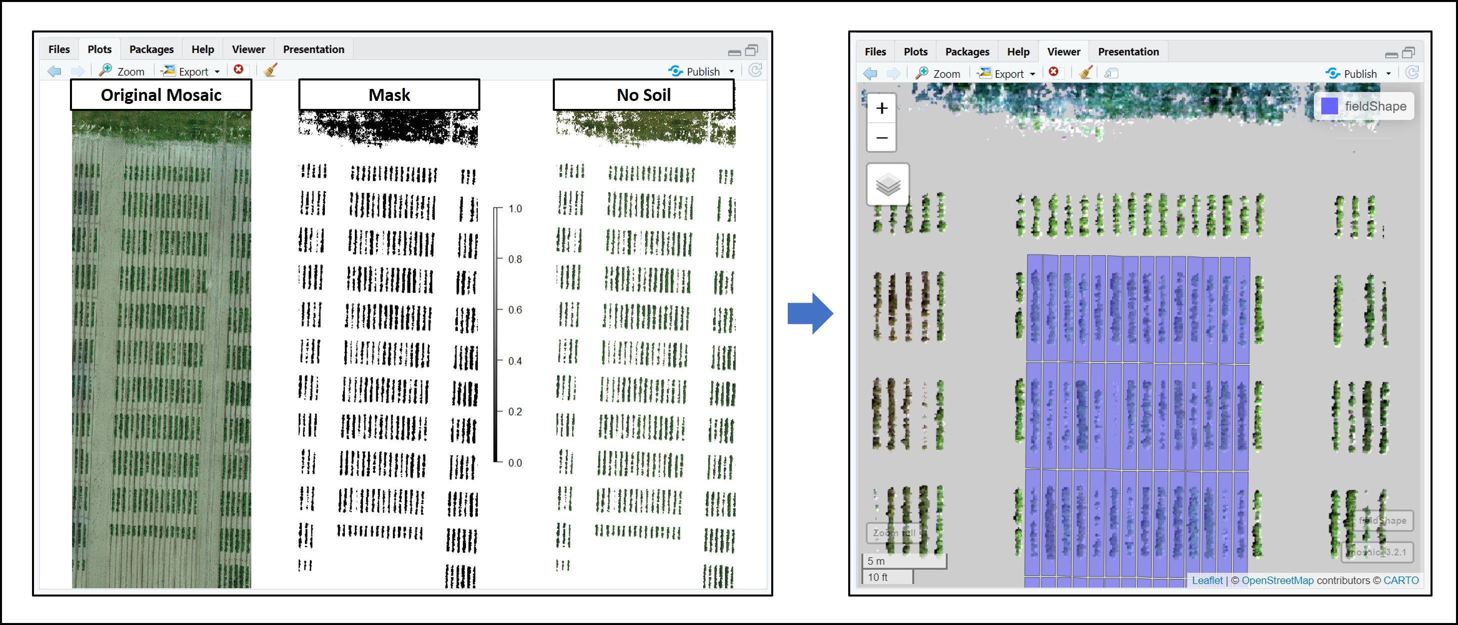
# Soil Mask (cluster 2) to remove soil effect from the mosaic using FIELDimageR::fieldMask :
soil<-Test.kmean==2
Test.RemSoil<-fieldMask(Test.Indices,
                        mask = soil) 
fieldView(Test.RemSoil$newMosaic,
          fieldShape = editShape,
          type = 2,
          alpha_grid = 0.2)

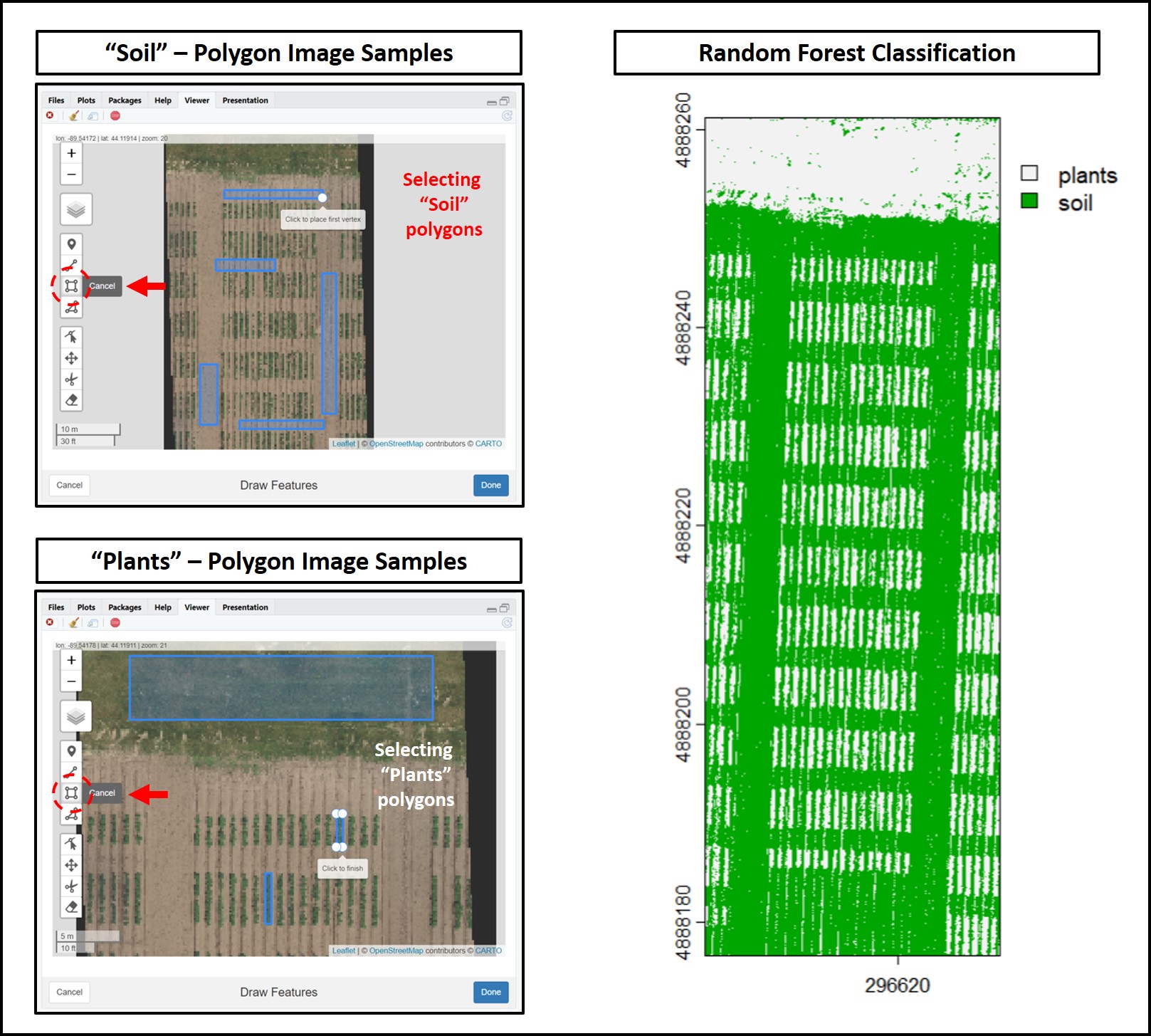
Option 02 is the new function [fieldSegment]. This function uses samples of images and machine learning algorithms for pixel classification (Supervised method). There are two models included Random Forest (default) and cart. Initially, users need to create training samples by using fieldView function by enabling the editor option to digitize spatial object (e.g. soil, plant, shadow etc.). For instance, users need to utilize the draw polygon or draw rectangle tool in the editor. The mapedit objects have 0.000001 degree spatial resolution, about 10 cm at the equator (Source: r-spatial/mapedit#63). For images with coarse spatial resolution, this level of precision won't significantly affect digitization accuracy. However, for UAV images with high spatial resolution, this precision (around 10 cm) can significantly impact the accuracy of digitization. Therefore, using the pointer tool in the editor for digitizing small objects like flowers could potentially lead to inaccuracies in the digitization position. For accurate results, prefer to draw polygon or rectangle tools in the editor for digitizing larger size objects. For digitizing smaller objects(e.g. flowers) users can use QGIS software and use it for further analysis in R.

### Option_02 = Using fieldSegment()

# Digitize soil object by drawing polygons at least 5-6 large polygon uniformly distributed
soil<-fieldView(mosaic = Test, editor = TRUE) #generate random 200 points for soil class
soil<-st_as_sf(st_sample(soil, 200))
soil$class<-'soil'

# Digitize plants object by drawing polygons. The number of polygon will depends upon the number of training points to be generated.
plants<-fieldView(mosaic = Test, editor = TRUE)
plants<-st_as_sf(st_sample(plants, 200)) #generate random 200 points for plants class
plants$class<-'plants'

#similarly you can digitize shadow, other objects by using draw polygon tool of editor
training_sam<-rbind(soil,plants)

# Random Forest model:
classification<-fieldSegment(mosaic = Test, 
                             trainDataset = training_sam)

# To display results of classification from randomForest
classification$sup_model
classification$pred
classification$rastPred
fieldView(classification$rastPred)
plot(classification$rastPred)

# Creating a mask to remove soil from the original image:
soil<-classification$rastPred=="soil"
Test.RemSoil<-fieldMask(Test.Indices,
                        mask = soil) 
fieldView(Test.RemSoil$newMosaic,
          fieldShape = editShape,
          type = 2,
          alpha_grid = 0.2)

Option 03 is the traditional way to remove soil using the function FIELDimageR::fieldMask from FIELDimageR package (Thresholding Method).

# Option_03 = Using the traditional FIELDimageR::fieldMask()
Test.RemSoil<-fieldMask(Test.Indices) 
fieldView(Test.RemSoil$newMosaic,
          fieldShape = editShape,
          type = 2,
          alpha_grid = 0.2)

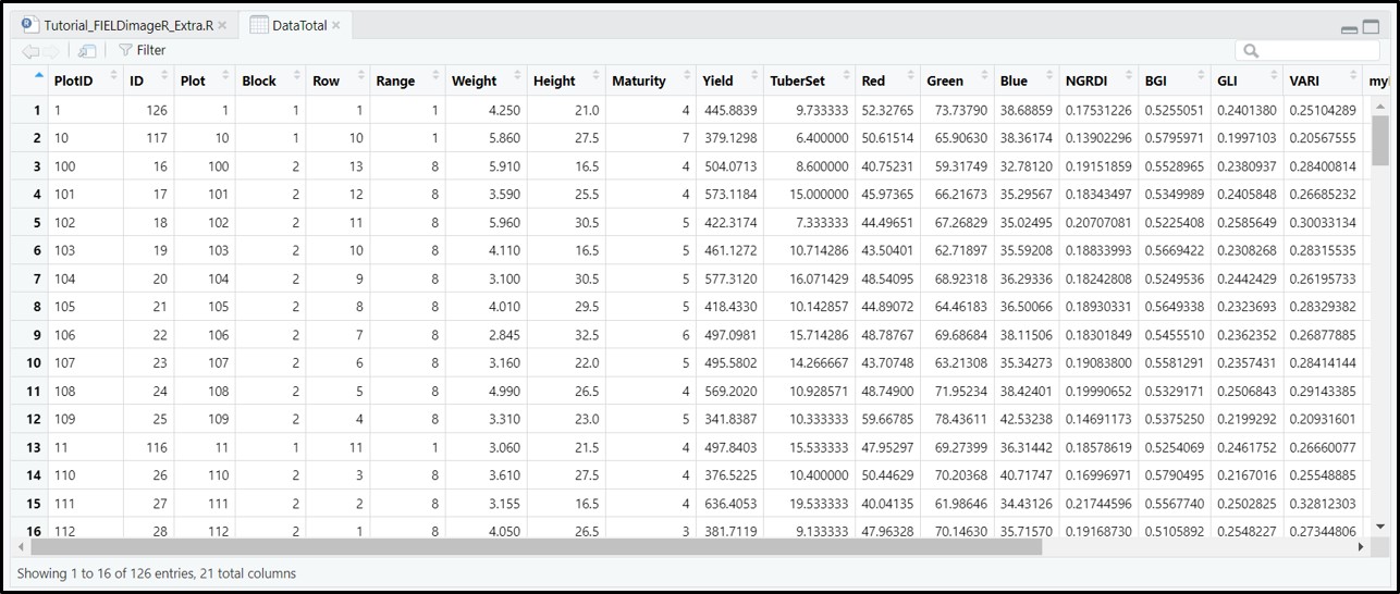
7. Extracting data from field images

The function aggregate from stars was adapted for agricultural field experiments through function fieldInfo_extra.

DataTotal<- fieldInfo_extra(mosaic = Test.RemSoil$newMosaic,
                    fieldShape = editShape, 
                    fun = mean)
DataTotal

8. Vizualizing extracted data

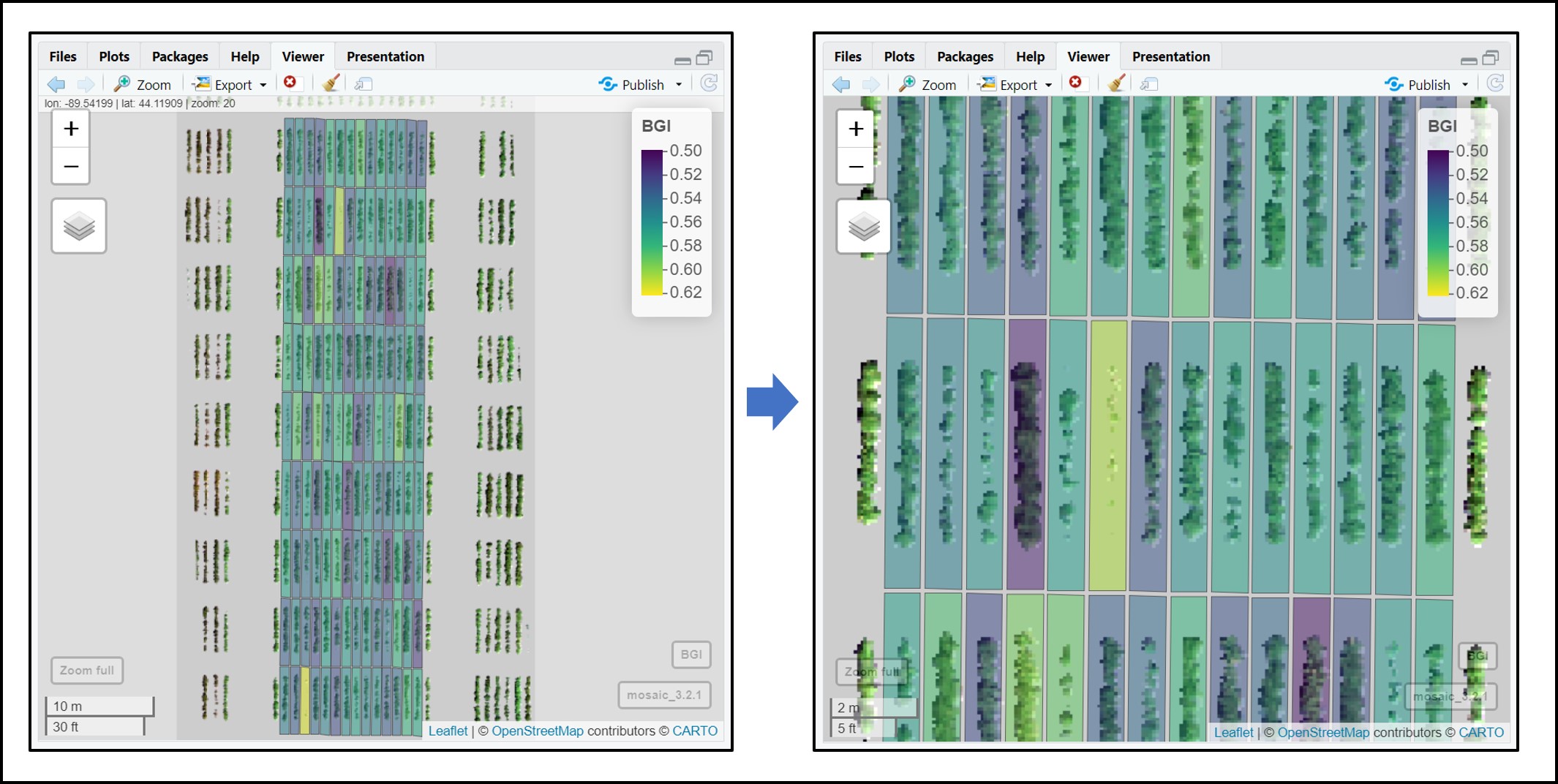
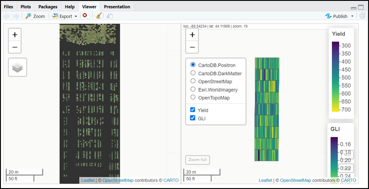
There are different ways to use the function fieldView to visualize and interpret extracted data.

# Visualizing single layer vegetation index 'BGI': 
fieldView(mosaic = Test.RemSoil$newMosaic,
          fieldShape = DataTotal,
          plotCol = "BGI",
          type = 2,
          alpha_grid = 0.6)

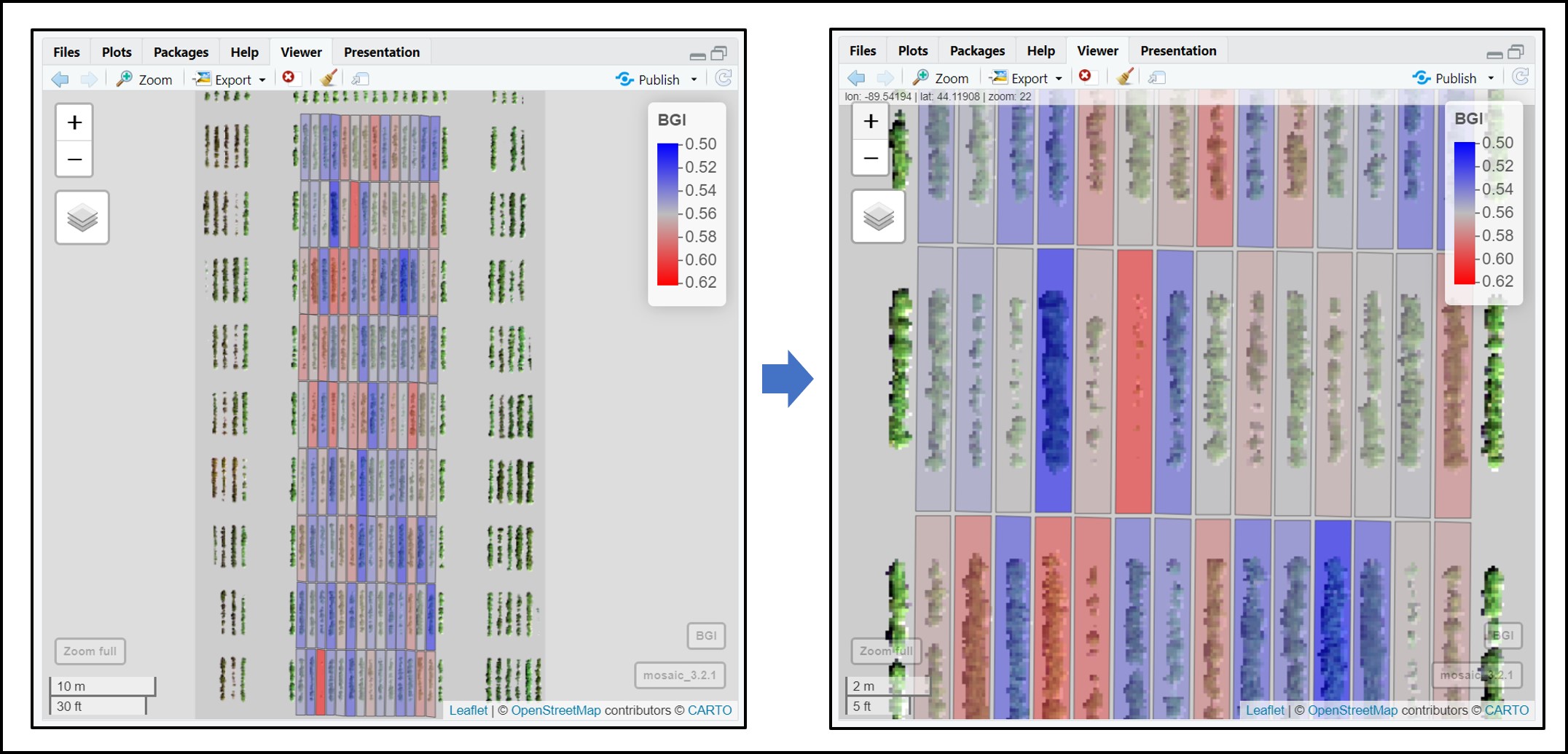
# Applying different color schemes to paint plots in the fieldShape file. An example using extracted values for 'BGI': 
fieldView(mosaic = Test.RemSoil$newMosaic,
          fieldShape = DataTotal,
          plotCol = "BGI",
          col_grid = c("blue", "grey", "red"),
          type = 2,
          alpha_grid = 0.6)

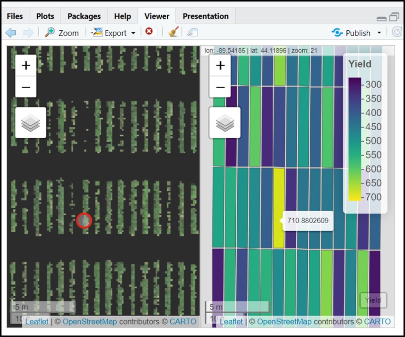
# Coloring fieldShape file using 'Yield' to highlight plots: 
fieldView(mosaic = Test.RemSoil$newMosaic,
          fieldShape = DataTotal,
          plotCol = c("Yield"),
          type = 1)

# Coloring fieldShape file using more traits: 
fieldView(mosaic = Test.RemSoil$newMosaic,
          fieldShape = DataTotal,
          plotCol = c("Yield","GLI"),
          type = 1)

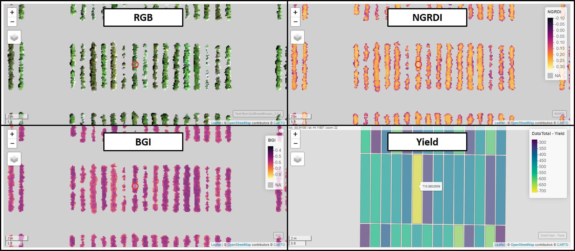
# Syncronizing individual layers:
library(leafsync)
m1<-viewRGB(Test.RemSoil$newMosaic)
m2<-mapview(Test.RemSoil$newMosaic$NGRDI,layer.name="NGRDI")
m3<-mapview(Test.RemSoil$newMosaic$BGI,layer.name="BGI")
m4<-mapview(DataTotal,zcol="Yield")
sync(m1,m2,m3,m4)

9. Saving output files and opening them in the QGIS

# Saving Data.csv (You can remove the 'geometry' info):
write.csv(as.data.frame(DataTotal)[,-dim(DataTotal)[2]],"DataTotal.csv",col.names = T, row.names = F)

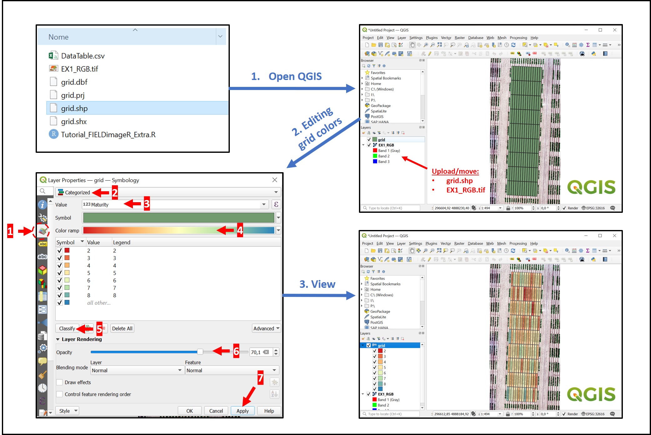
# Saving grid fieldShape file:
st_write(DataTotal,"grid.shp")

# To read saved.shp object:
Saved_Grid= st_read("grid.shp")

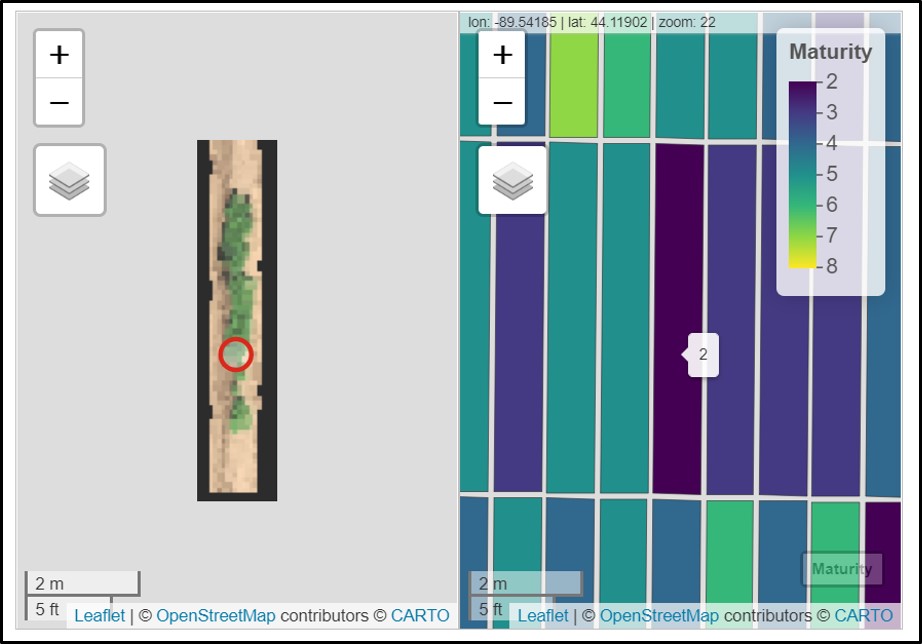
The saved "grid.shp" can be opened on others GIS softwares as QGIS. Users can easily upload the orthomosaic and grid.shp by holding the file from the folder and dragging it to a new project at QGIS. There are different visualization possibilities in QGIS. In the example below, each plot was identified according to the maturity score. However, any vegetation index calculated with FIELDimageR::fieldIndex can be visualized as well.

10. Cropping individual plots and saving

Many times when developing algorithms it is necessary to crop the mosaic using the plot fieldShape as a reference and sort/store cropped plot images on specific folders. For instance, the function fieldCrop_grid allows cropping plots and identification by 'plotID'. The user also can save each plot according to a 'classifier' logic (Attention: a column in the 'fieldShape' with the desired classification must be informed). In the example below, each plot in the 'Test.Indices' mosaic is being cropped according to the 'editShape' grid file, identified by the information in the 'plot' column, and stored/saved in specific folders with different levels of Maturity the 'classifier'.

# Saving plot images format .jpg according to 'Maturity': 
Field_plot_grids<- fieldCrop_grid(mosaic = rast(Test.Indices),
                                  fieldShape = editShape, 
                                  classifier = "Maturity", 
                                  plotID = "Plot",
                                  format = '.jpg',
                                  output_dir = "./")

# Visualizing plot "#21"
fieldView(Field_plot_grids$'21')

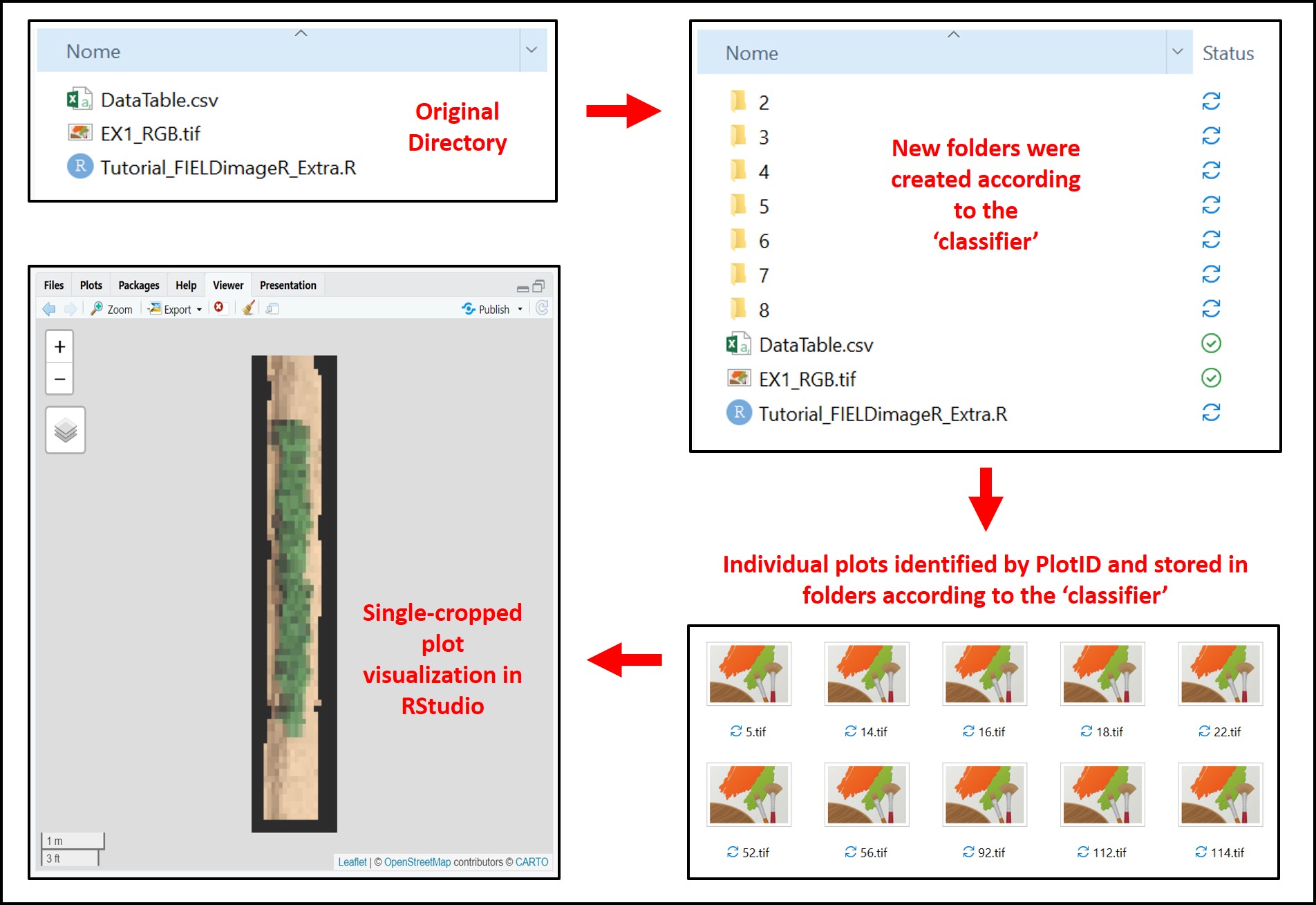
# Saving plot images format .tif according to 'Maturity':
Field_plot_grids<- fieldCrop_grid(mosaic = rast(Test.Indices),
                                  fieldShape = editShape, 
                                  classifier = "Maturity", 
                                  plotID = "Plot",
                                  format = '.tif',
                                  output_dir = "./")

# Reading .tif file and visualizing single plots with fieldView()
tif<-rast("./2/21.tif")
fieldView(mosaic = tif,
          fieldShape = editShape,
          plotCol ="Maturity")

Google Groups Forum

This discussion group provides an online source of information about the FIELDimageR package. Report a bug and ask a question at:

Developers

Help improve FIELDimageR.Extra pipeline. The easiest way to modify the package is by cloning the repository and making changes using R projects.

If you have questions, join the forum group at https://groups.google.com/forum/#!forum/fieldimager

Try to keep commits clean and simple

Submit a pull request with detailed changes and test results.

Let's work together and help more people (students, professors, farmers, etc) to have access to this knowledge. Thus, anyone anywhere can learn how to apply remote sensing in agriculture.

Licenses

The R/FIELDimageR package as a whole is distributed under GPL-3 (GNU General Public License version 3).

Citation

Pawar P & Matias FI.* FIELDimageR.Extra. (2023) (Submitted)
Matias FI, Caraza-Harter MV, Endelman JB. FIELDimageR: An R package to analyze orthomosaic images from agricultural field trials. The Plant Phenome J. 2020; https://doi.org/10.1002/ppj2.20005

Author

Popat Pawar

Filipe Matias

Acknowledgments

OpenDroneMap

Phenome-Force Channel

r-spatial community

jenniferlopes / fieldimager.extra Goto Github PK

fieldimager.extra's Introduction

FIELDimageR.Extra: An package with new tools to support FIELDimageR software on evaluating GIS images from agriculture field trials using R.

Resources

Installation

Using R/FIELDimageR.Extra

1. First steps

2. Loading mosaics and visualizing

3. Building the plot shapefile (Zoom)

4. Editing plot shapefile (Zoom)

5. Building vegetation indices

6. Removing the soil effect

7. Extracting data from field images

8. Vizualizing extracted data

9. Saving output files and opening them in the QGIS

10. Cropping individual plots and saving

Google Groups Forum

Developers

Licenses

Citation

Author

Acknowledgments

fieldimager.extra's People

Contributors

Recommend Projects

Recommend Topics

Recommend Org