
SParry is a shortest path calculating Python tool using some algorithms with CUDA to speedup.
It's developing.
SParry is a shortest path calculation toolkit, the main shortest path algorithms, including Dijkstra, Bellman-Ford, Delta-Stepping, and Edge-Based, are encapsulated. A parallel accelerated version based on CUDA is provided to improve development efficiency.
At the same time, SParry can divide the graph data into parts, and solve it more quickly than using the CPU when the graph is too large to put it in the GPU directly.
The following is the environment that passed the test in the development experiment.
You can also see them in requirements.txt.
Python Version
python3.6
python3.7
Plantform
Windows
Linux
Requirements
cyaron==0.4.2 networkx==2.5 numpy==1.19.4 pycuda==2019.1.2 pynvml==8.0.4
Download the file package directly and run the calc interface function in the main directory.
**It's not a release version currently, so it cannot be installed with pip, and the development structure is not yet perfect. **

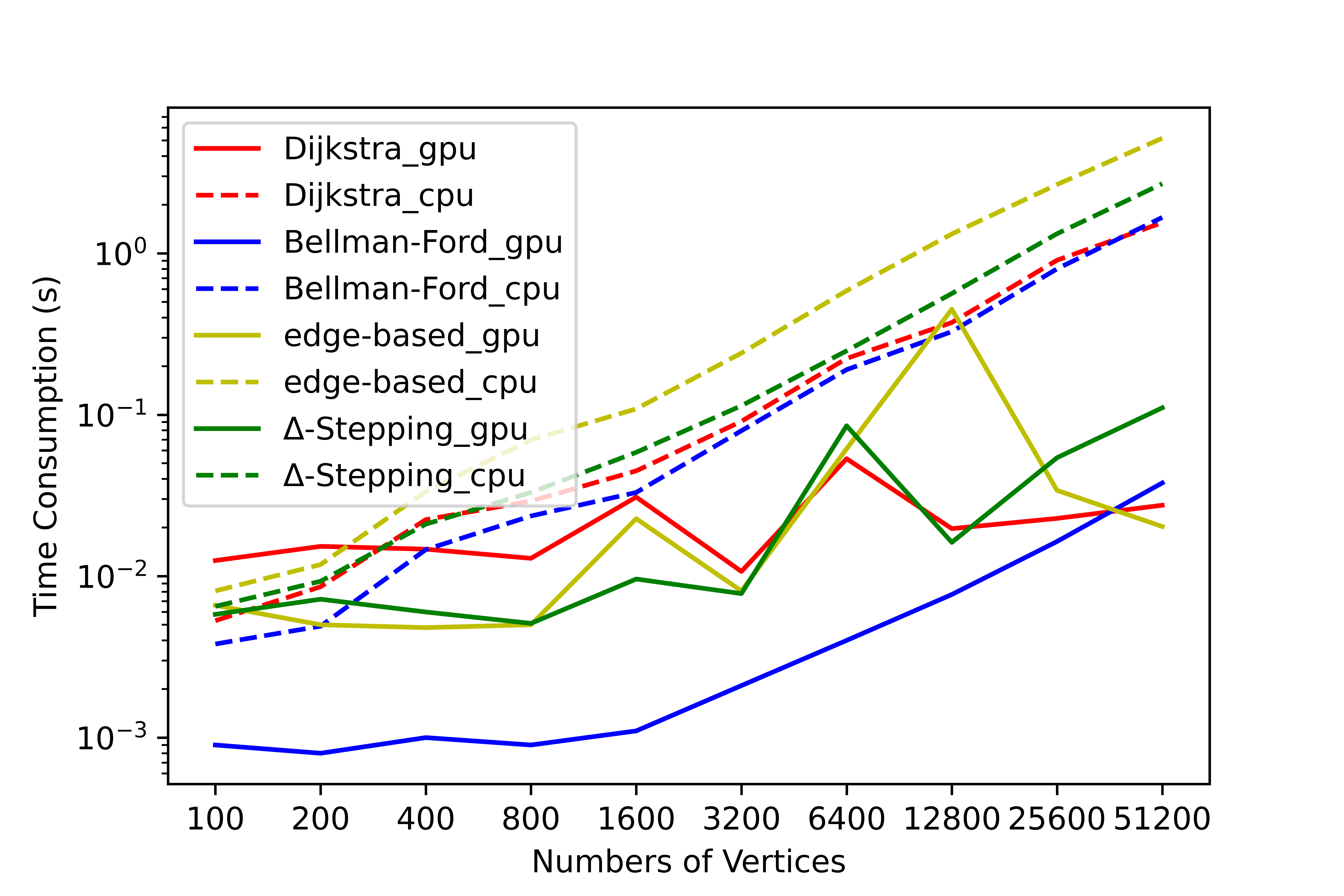
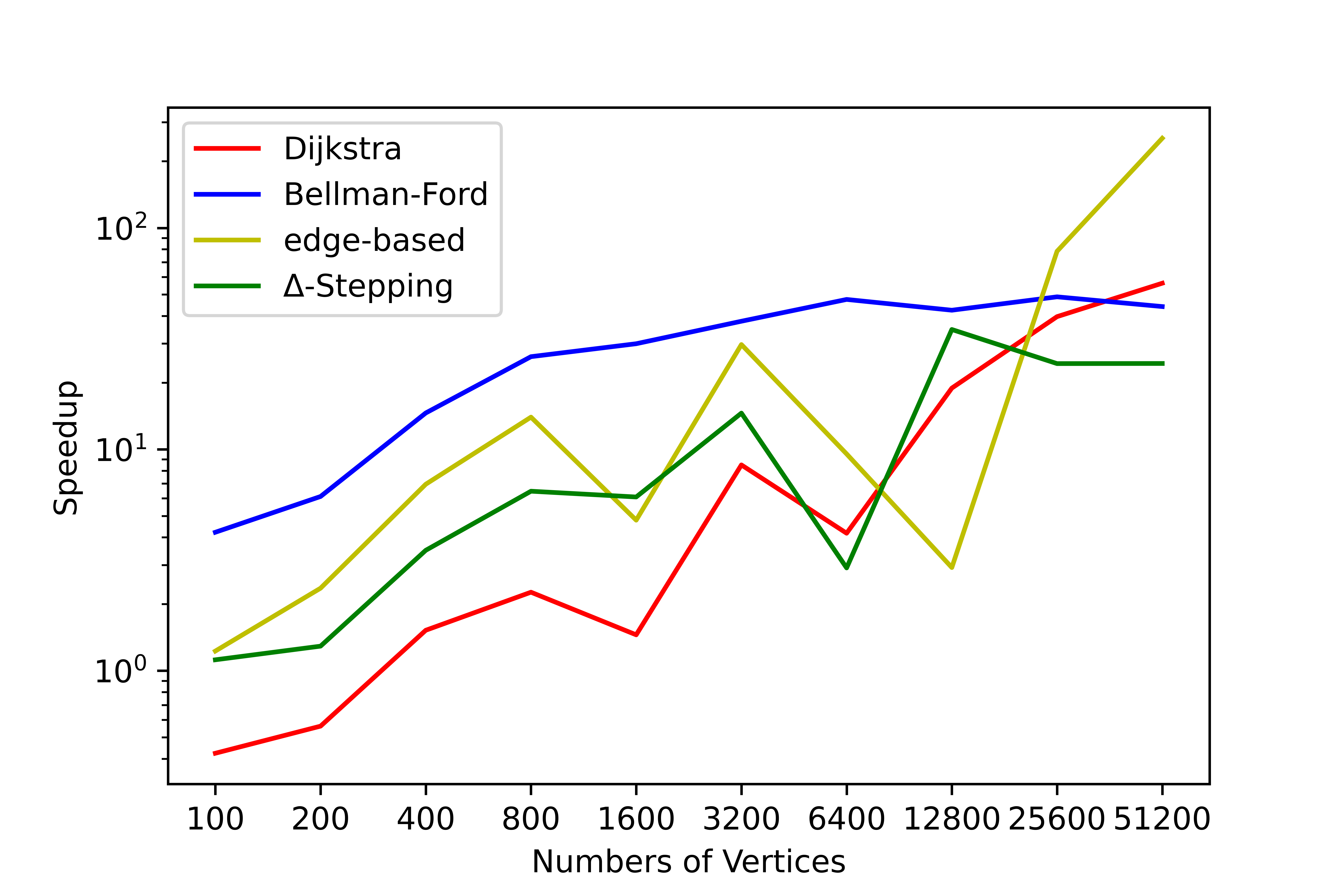
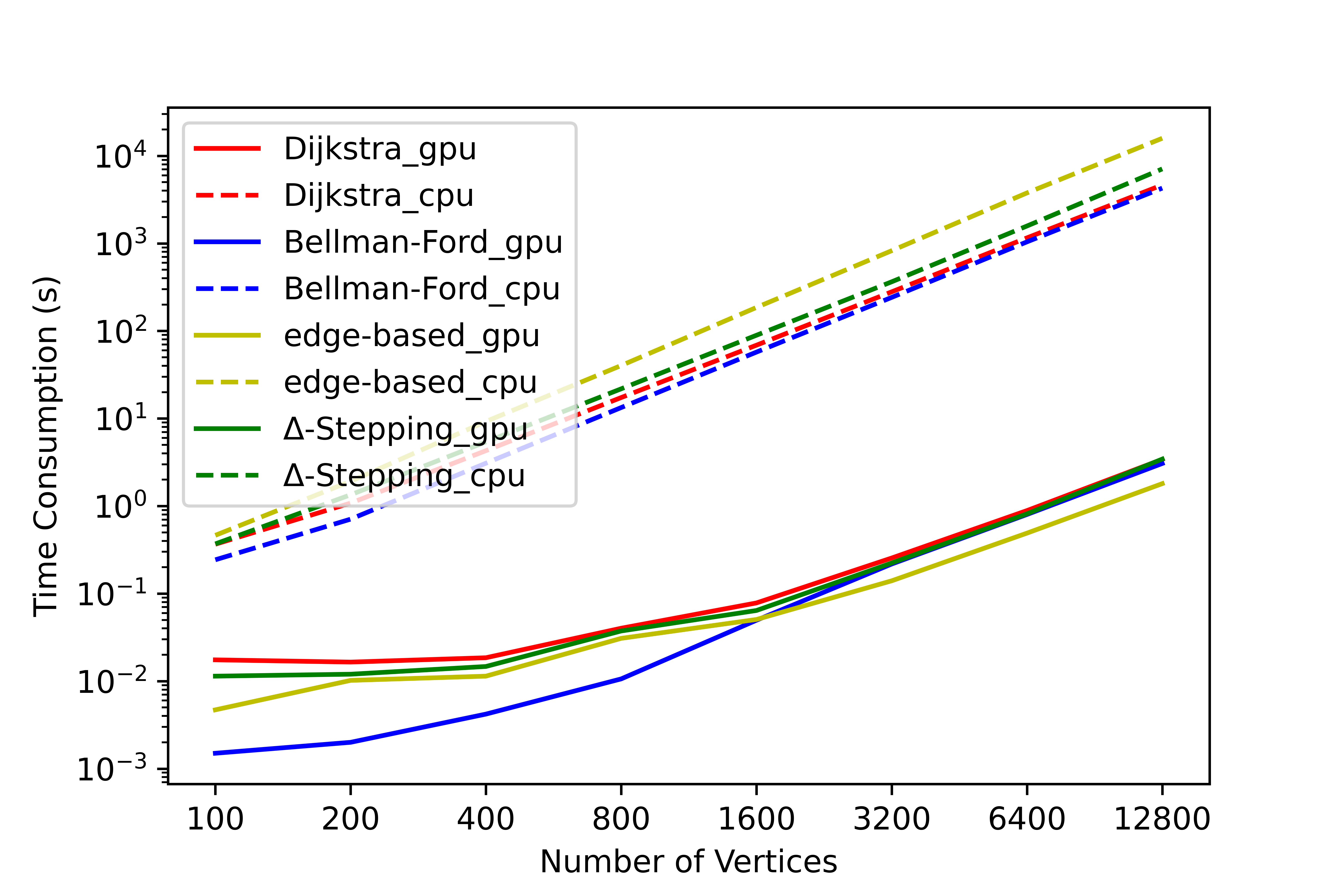
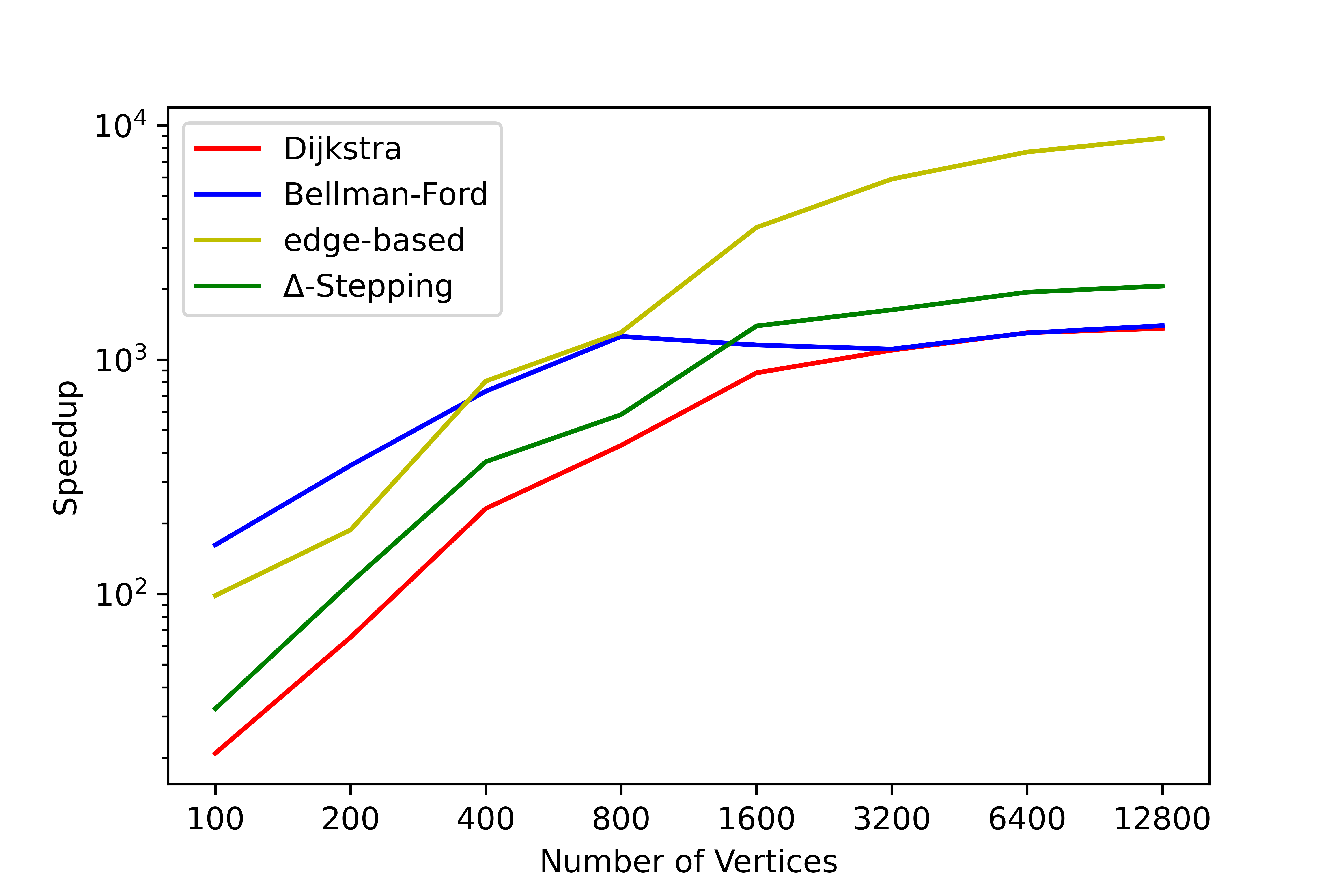
We have conducted a lot of tests on this tool, and no errors occurred in the test results. We have counted the time consumption and serial-parallel speedup ratio of each algorithm on some graphs to solve the single-source shortest path (SSSP) and all-pairs shortest path (APSP). The following shows the time variation of each algorithm with the number of nodes when the average degree is 4, please refer to SParry/testResult .
This section is an introduction to help beginners of SParry get started quickly. You can also see these in demo.py.
cd XXX/SParry/When your graph data is in memory and meets the adjacency-matrix data requirements, you can import your data as below to quickly calculate the results.
>>> from calc import calc
>>> import numpy as np
>>> from pretreat import read
>>>
>>> matrix = np.array([[0,1,2,3],[1,0,2,3],[2,2,0,4],[3,3,4,0]], dtype = np.int32) # the data of the adjacency matrix
>>> matrix # simulate graph data that already has an adjacency matrix
array([[0, 1, 2, 3],
       [1, 0, 2, 3],
       [2, 2, 0, 4],
       [3, 3, 4, 0]], dtype=int32)
>>>
>>> graph = read(matrix = matrix, # the data passed in is the adjacency matrix
...              method = "dij", # the calculation method uses Dijkstra
...              detail = True # record the details of the graph
...             ) # process the graph data
>>>
>>> res = calc(graph = graph, # class to pass in graph data
...            useCUDA = True, # use CUDA acceleration
...            srclist = 0, # set source to node 0
...            )
>>>
>>> res.dist # output shortest path
array([0, 1, 2, 3], dtype=int32)
>>>
>>> print(res.display()) # print related parameters

[+] the number of vertices in the Graph:                n = 4,
[+] the number of edges(directed) in the Graph:         m = 16,
[+] the max edge weight in the Graph:                   MAXW = 4,
[+] the min edge weight in the Graph:                   MINW = 0,
[+] the max out degree in the Graph:                    degree(0) = 4,
[+] the min out degree in the Graph:                    degree(0) = 4,
[+] the average out degree of the Graph:                avgDegree = 4.0,
[+] the directed of the Graph:                          directed = Unknown,
[+] the method of the Graph:                            method = dij.


[+] calc the shortest path timeCost = 0.017 sec
>>>
>>> res.drawPath() # The red line indicates that this edge is on the shortest path; the orange vertex is the source vertex; the arrow indicates the direction of the edge; and the number on the edge indicates the edge weight.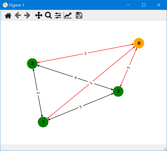
When your graph data is in memory and compliant with the CSR data requirements, you can import your data as below to quickly calculate the results.
>>> from calc import calc
>>> import numpy as np
>>> from pretreat import read
>>>
>>> CSR = np.array([np.array([0, 2, 3, 4, 4]),
...                 np.array([1, 2, 3, 1]),
...                 np.array([1, 3, 4, 5])])
>>> CSR # simulation already has CSR format is graph data
array([array([0, 2, 3, 4, 4]), array([1, 2, 3, 1]), array([1, 3, 4, 5])],
      dtype=object)
>>>
>>> graph = read(CSR = CSR, # The data type passed in is CSR
...              method = "delta", # The algorithm used is delta-stepping
...              detail = True) # record the details of the graph
>>> # calculated shortest path
>>> res = calc(graph = graph, # the incoming graph data class
...            useCUDA = True, # use CUDA parallel acceleration
...            srclist = 0) # source point is node 0
>>>
>>> res.dist # output shortest path
array([0, 1, 3, 5], dtype=int32)
>>>
>>> print(res.display()) # print related parameters

[+] the number of vertices in the Graph:                n = 4,
[+] the number of edges(directed) in the Graph:         m = 4,
[+] the max edge weight in the Graph:                   MAXW = 5,
[+] the min edge weight in the Graph:                   MINW = 1,
[+] the max out degree in the Graph:                    degree(0) = 2,
[+] the min out degree in the Graph:                    degree(3) = 0,
[+] the average out degree of the Graph:                avgDegree = 1.0,
[+] the directed of the Graph:                          directed = Unknown,
[+] the method of the Graph:                            method = delta.


[+] calc the shortest path timeCost = 0.007 secWhen your graph data is in memory and compliant with the edgeSet data requirements, you can import your data as below to quickly calculate the results.
>>> from calc import calc
>>> import numpy as np
>>> from pretreat import read
>>>
>>> edgeSet = [[0, 0, 2, 1], # start point of each edge
...            [1, 3, 1, 3], # the end point of each edge
...            [1, 2, 5, 4]] # weights of each edge
>>>
>>> edgeSet # simulation already has edgeSet format is graph data
[[0, 0, 2, 1], [1, 3, 1, 3], [1, 2, 5, 4]]
>>>
>>> graph = read(edgeSet = edgeSet, # the incoming graph data is edgeSet
...              detail = True) # need to record the data in the graph
>>> # calculated shortest path
>>> res = calc(graph = graph, # the incoming graph data class
...            useCUDA = False, # sse CPU serial computation
...            srclist = 0) # source point is node 0
>>> res.dist # output shortest path
array([         0,          1, 2139045759,          2], dtype=int32)
>>>
>>> print(res.display()) # print related parameters

[+] the number of vertices in the Graph:                n = 4,
[+] the number of edges(directed) in the Graph:         m = 4,
[+] the max edge weight in the Graph:                   MAXW = 5,
[+] the min edge weight in the Graph:                   MINW = 1,
[+] the max out degree in the Graph:                    degree(0) = 2,
[+] the min out degree in the Graph:                    degree(3) = 0,
[+] the average out degree of the Graph:                avgDegree = 1.0,
[+] the directed of the Graph:                          directed = Unknown,
[+] the method of the Graph:                            method = dij.


[+] calc the shortest path timeCost = 0.0 secWhen your graph data is stored in a file and meets the data requirements (file data) , you can also pass in a file to calculate the shortest path.
The file in this example is as follows, test.txt .
4 6
0 1 1
0 2 2
0 3 3
1 2 2
1 3 3
2 3 4
code is below:
>>> from calc import calc
>>> import numpy as np
>>> from pretreat import read
>>>
>>> filename = "./data/test.txt" # the path to the file where the graph data is stored
>>> graph = read(filename = filename, # the data passed in is the file
...              method = "spfa", # the algorithm used is spfa
...              detail = True, # record the details of the graph
...              directed = False) # the graph is an undirected graph
>>> # calculated shortest path
>>> res = calc(graph = graph, # the incoming graph data class
...            useCUDA = True, # use CUDA parallel acceleration
...            srclist = 0) # source point is node 0
>>>
>>> res.dist # output shortest path
array([0, 1, 2, 3], dtype=int32)
>>>
>>> print(res.display()) # print related parameters

[+] the number of vertices in the Graph:                n = 4,
[+] the number of edges(directed) in the Graph:         m = 12,
[+] the max edge weight in the Graph:                   MAXW = 4,
[+] the min edge weight in the Graph:                   MINW = 1,
[+] the max out degree in the Graph:                    degree(0) = 3,
[+] the min out degree in the Graph:                    degree(0) = 3,
[+] the average out degree of the Graph:                avgDegree = 3.0,
[+] the directed of the Graph:                          directed = False,
[+] the method of the Graph:                            method = spfa.


[+] calc the shortest path timeCost = 0.002 sec
>>> res.drawPath() # The red line indicates that this edge is on the shortest path; the orange vertex is the source vertex; the arrow indicates the direction of the edge; and the number on the edge indicates the edge weight.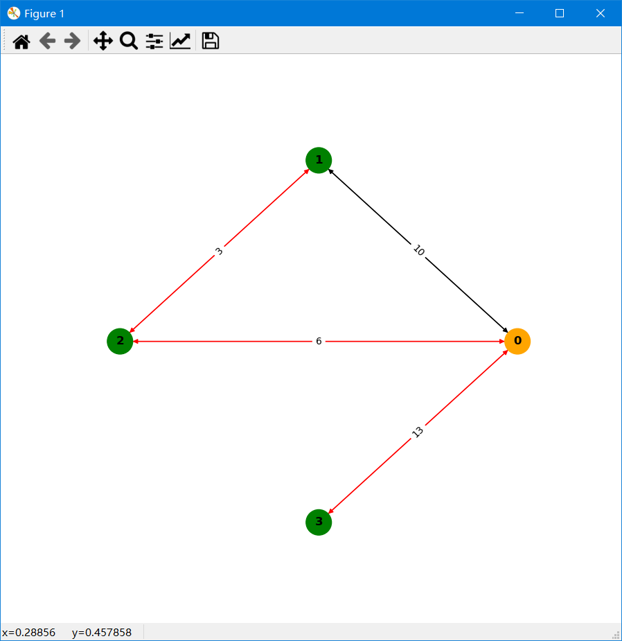
Pseudocodes can be found at: pseudocode.
Please see the developer tutorials for more information.