Genetic algorithms applied in Computer Fluid Dynamics for multiobjective optimization
This is a Senior Thesis developed for the BSc Aerospace Engineering at the University of Leon. However, this project was done at the University of Vermont during an exchange program. The main purpose of this thesis was to couple a metaheuristic optimization method, such as genetic algorithm (GA), with aerospace cases simulated with computer fluid dynamics (CFD) that have multiple objectives (MO).
| Author: | Javier Lobato Perez |
|---|---|
| Advisors: | Yves Dubief and Rafael Santamaria |
| Institution: | University of Vermont - Mechanical Engineering department |
The project required some software to be present on the computer in order to properly run it. The requisites are python (version used was 3.6.1) (with either jupyter notebook or jupyter lab to execute the notebooks and understand the basics of the process), OpenFOAM (version 5.00 was used) and paraView (version 5.4.0). Required Python packages are the basic numpy, matplotlib, scipy, numba, sympy... However optunity, tdqm and prettytable are required to run every notebook. The operating system used for Python bash commands and scripting was Ubuntu 16.04 LTS. Compatibility with other OS has not been tested.
This readme file is structured in two parts. The first one is a quick overview of the project, showing how to further use the code, the analyzed cases, the development of the code and a brief description of all the terms. However, in the second part, there is a folder by folder analysis that lists the scripts and code of each folder with a brief description to find something in the future with a quick search.
The full report of the project is located at https://github.com/jlobatop/senior-thesis-tex.
Table of Contents
QUICK OVERVIEW
This repository has all the files of the project from the very beginning. It all started with a search of interesting topics to dig a little further: from the Lorena Barba's awesome 12 steps to Navier Stokes. course in Python to different mesh generation tools and airfoil parametrization [1]. Finally, the objective was to use a genetic algorithm (specifically the NSGA-II: Non-dominated Sorting Genetic Algorithm II [2] ) for multiobjective optimization of different computer fluid dynamic cases.
The basic of genetic algorithms must be briefly described before explaining the project. A genetic algorithm is a metaheuristic stochastical global optimization method based on populations: an initial generation is randomly generated and evaluated, the fitness (a measure of how 'good' does an individual performs within the population) is computed and the individuals with higher fitness are randomly combined and mutated, obtaining a new generation with new individuals (that are again evaluated, looping until a stop condition is reached). The main idea is that high fitness parents will give high fitness offspring [3] (the fitness value doesn't always increase, but it will not decrease). GA are a good approach to a CFD optimization because no gradient information is required and the structure of the fitness function is fairly simple. Thus, each individual will be a CFD simulation that depends on some search space variables (change in boundary conditions, mesh, ...) and it will return (amongst a lot of data) some function space values outputs of the CFD simulation. Each individual of the GA is defined with search space variables and the values of the function space will be used as fitness value, trying to maximize or minimize it. Multiobjective is referred to the kind of optimization that tries to maximize not one but more objectives at the same time. Usually, those objectives are in trade-off (when one is optimized the other has its least optimum value), so one single solution is unfeasible. The Pareto front is the set of possible solutions that optimize all objectives as much as possible. There are a lot of genetic algorithms designed for multiobjective optimization (VEGA [4], MOGA [5], NSGA-II [2], DMOEA [6], ...), but the NSGA-II was chosen specially for being a well-tested method, efficient, with a straightforward implementation and without user-defined parameters (that usually condition the success of the optimization process).
At this point, the use of an already existing code of the NSGA-II was a plausible option: there are libraries as PyGMO or Platypus designed for multiobjective optimization in Python. However, as the fitness of the individuals will be determined from a CFD simulation with OpenFOAM, an automatic implementation using only Python was unfeasible (or at least, more complex than mixing Python and bash scripting). Thus, the NSGA-II was coded up in Python, first in jupyter notebooks (in order to see the different steps of the process) and then it was separated in Python scripts for the different phases of the project (initialization of the first generation, fitness evaluation of a generation, evolution of the generations (taking the fitness of the previous generation and applying selection, crossover and mutation) and problemSetup which includes the constraints of the problem). Other Python scripts may be required for the CFD post-processing of the case and data analysis, as well as pvbatch scripts for command line manipulation of the case in paraView.
The different scripts will refer to text files that store both the search space and the function space values for each generation and individuals. Those text files are the outputs of either a genetic algorithm script (search space values are the output of the evolution.py) or a CFD simulation (e.g., the lift and drag are the forces output of the OpenFOAM simulation). The basic structure of the folder tree before running the algorithm is:
case/
├── baseCase/
│   ├── 0/
│   ├── constant/
│   └── system/
├── run.sh
├── runGen.sh
├── problemSetup.py
├── initialization.py
├── fitness.py
└── evolution.py
As said, other scripts may be included if further analysis of the CFD simulation is required. Folder structure will noticeably get larger after the process, having something close to:
case/
├── gen0/
│   ├── ind0/
│   │   ├── 0/
│   │   ├── 1/
│   │   ├── ...
│   │   ├── system/
│   │   ├── constant/
│   │   ├── postProcessing/
│   │   ├── BMg0i0
│   │   ├── RUNg0i0
│   │   └── g0i0.OpenFOAM
│   ├── ind1/
│   │   └── ...
│   ├── ...
│   ├── ind$N/
│   │   └── ...
│   ├── popX1_0
│   ├── popX2_0
│   └── data/
│       ├── FITg0i0.txt
│       ├── FITg0i1.txt
│       └── ...
├── gen1/
│   └── ...
    ├── ...
├── gen$gL/
│   └── ...
├── data/
│   ├── gen0.txt
│   ├── gen1.txt
│   └── ...
├── baseCase/
│   ├── 0/
│   ├── constant/
│   └── system/
├── run.sh
├── runGen.sh
├── problemSetup.py
├── initialization.py
├── fitness.py
└── evolution.py
Not all folder are displayed, using $N as the number of individuals per generation and $gL as generation limit. Also, depending on the type of solver, more or less folders will be saved, having only folders 0/ and lastIteration for a steady-state solver and all timestep folders for a transient solver. BMg0i0 is the output of the blockMesh operation for the individual 0 of the generation 0 (just if it is needed for each individual). data/ folder in each generation may store also data as convergence plots (as both joukowsky cases) or plots over a line from paraView (diffuser case). The data used for the Python scripts is stored in case/data/, having a file for each generation that stores x1, x2, f1, f2 for each individual (having that x1 and x2 are the search space variables and f1 and f2 the objective functions).
After this brief description of the algorithm and folder structure (and given that documentation of the code is written inside each script), the analysis of the three studied cases will be introduced. If the already existing cases are run again, the individuals will vary due to the stochasticity of the algorithm, but the Pareto front should be close to the one shown below.
Vortex supression in a cylinder wake
A cylinder (amongst a lot of other objects) facing a stream may undergo vortex shedding under certain conditions. Vortex phenomena are associated with strong vibrations and oscillations that may cause structural damage to the object (especially if the frequency of the cylinder matches the natural frequency of the structure). In order to reduce it, different methods can be applied. In this case, a passive blowing & suction flow control mechanism (preferred against a blowing mechanism that will not have a zero net momentum in the flow) is located in the rear part of a cylinder following the next schematics:
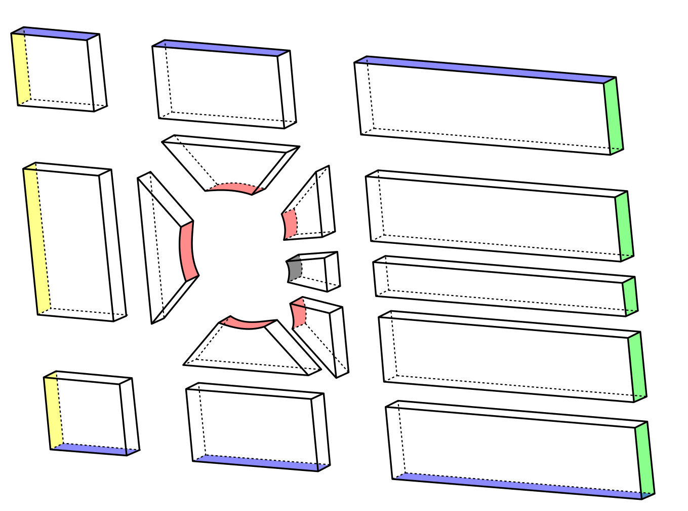
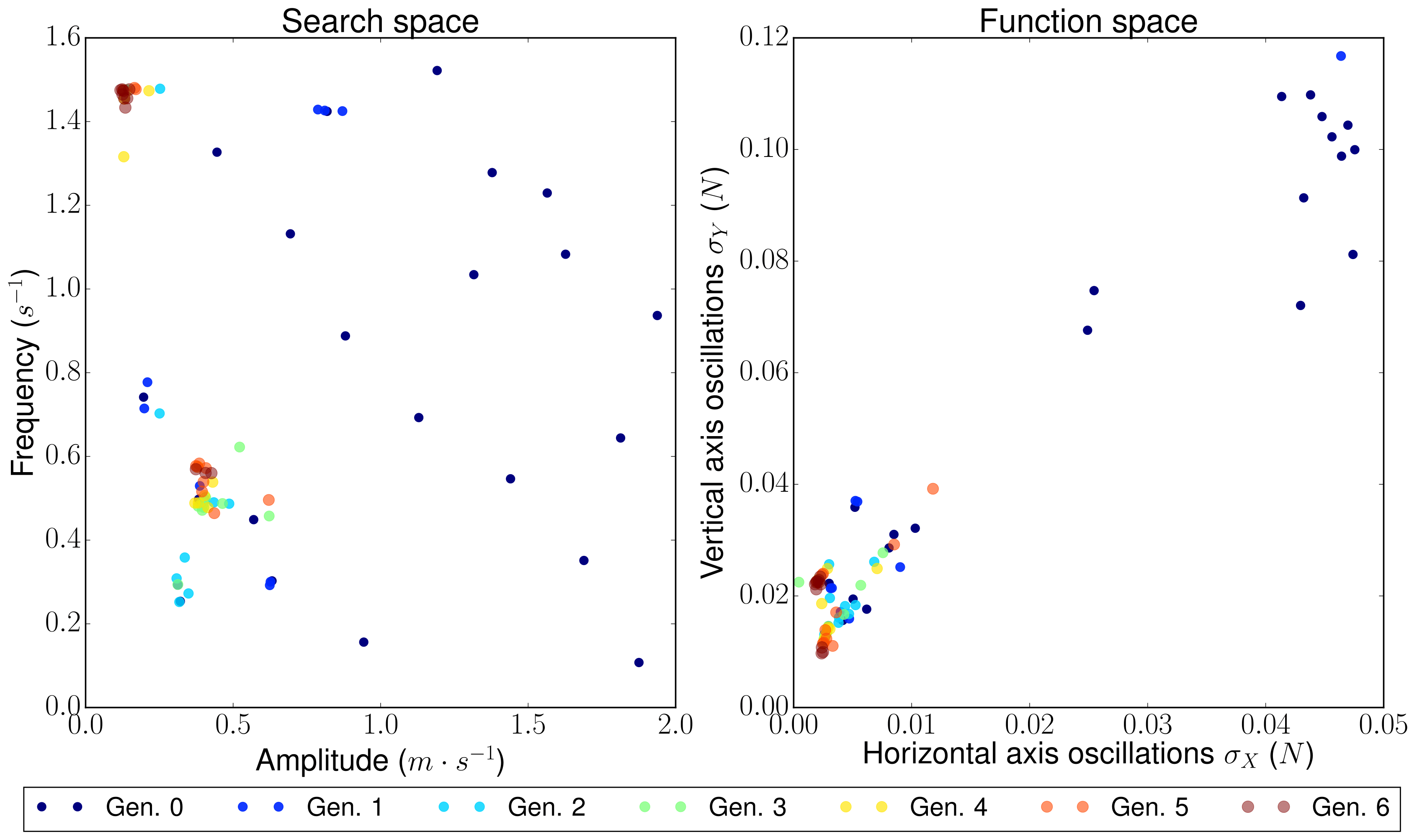
Mesh was constructed with blockMesh and faces correspond the different boundary conditions having that the grey face is the flowControl patch where the blowing & suction mechanism is located. The optimization problem has as search variables the amplitude and frequency of a sinusoidal wave that governs the flow control mechanism, that will (certainly) modify the flow field. The standard deviation of the force in the cylinder surface was decomposed in two axes (X and Y) and the objective is to minimize both at the same time. Standard deviation represents not the frequency of the oscillations but its amplitude (trying to reduce it as much as possible).
The individuals, in this case, don't make a Pareto front but they collapse into two solutions (or cluster of possible solutions). The next figure shows these results:
Some animations of the 'steady-state' of the oscillations ('steady-state' refers here to the time where oscillations where continuous and repetitive) may clarify the behavior of this cylinder:
- Cylinder with the flow control mechanism off:
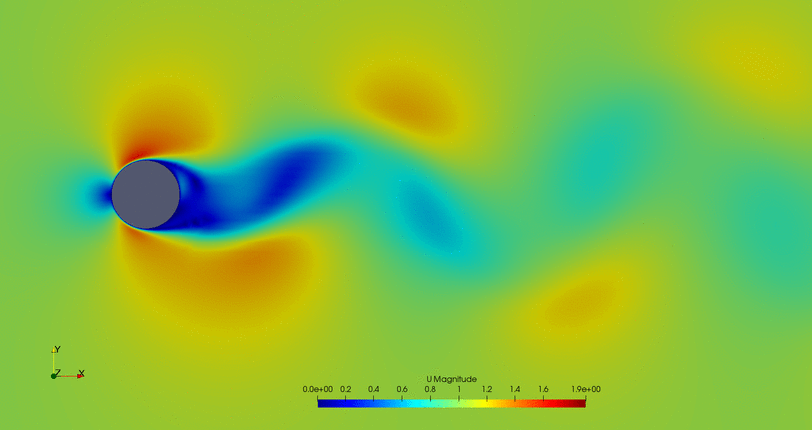
- Cylinder with the flow control on but a high fitness value (not efficient vortex cancellation):
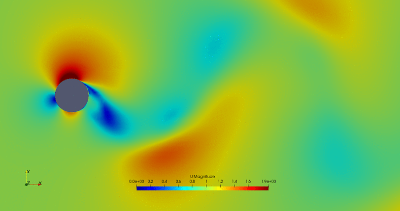
- Flow control of the first possible solution:
- Flow control of the second possible solution:
Convergence in two points may not be the the optimal solution, so further study of this case is required.
Diffuser inlet geometry design
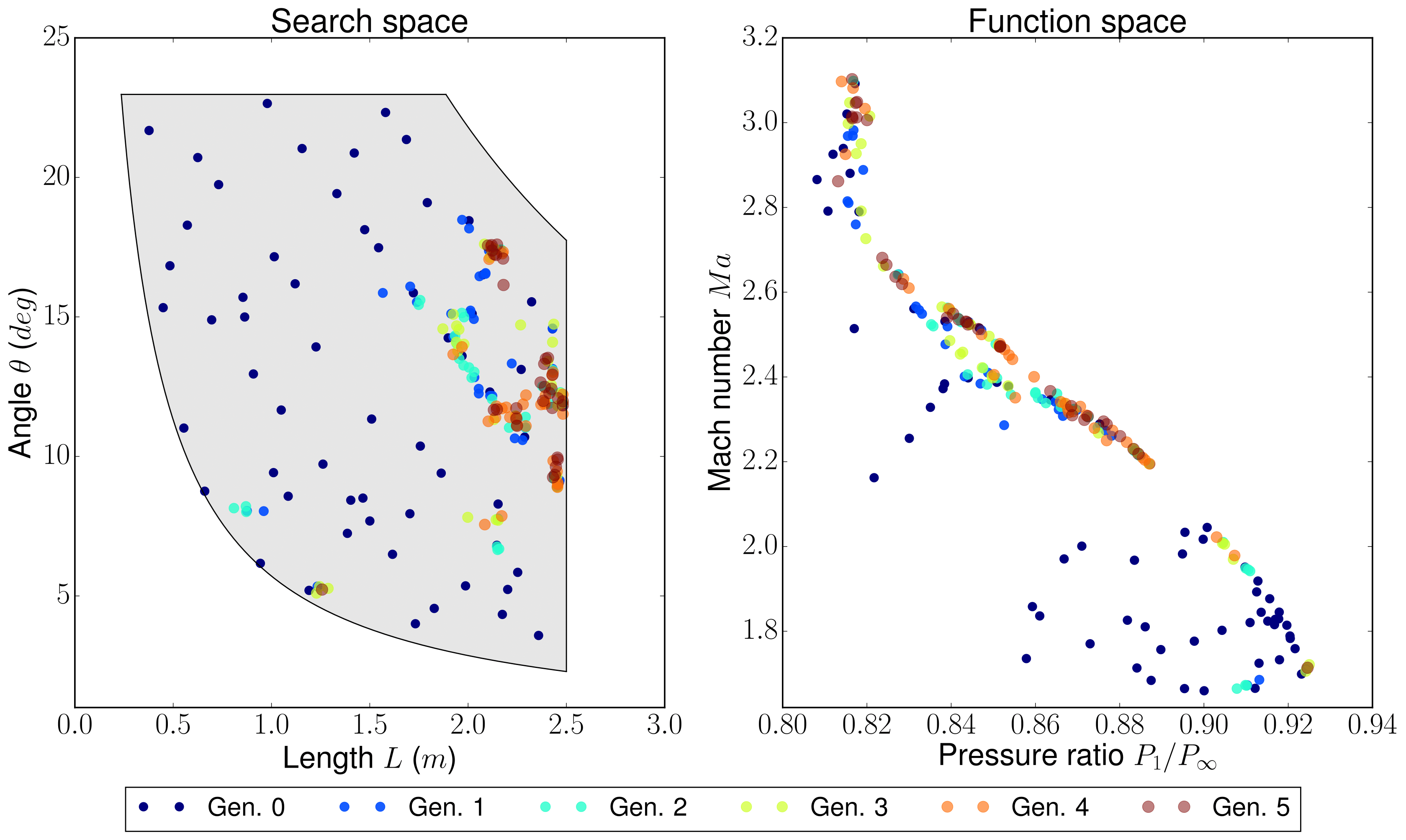
The inlet of a jet engine determines the state of all the other elements of the engine, having that the overall efficiency will decrease if the diffuser performance it is not on the most optimum value. To increase the efficiency of a diffuser, the pressure ratio between freestream and diffuser outlet must be as high as possible (having a low entropy generation due to supersonic shock waves). The performance of a combustion chamber may also be improved if the Mach number at its inlet is maximum. Thus the function space functions are Mach at the diffuser outlet (supposing no turbomachinery between diffuser and combustion chamber) and the pressure ratio (both will try to be the maximum). The search space variables are the length (L) and angle (theta) of the inlet of the diffuser as depicted by the next figure:

In this case, the results form a Pareto front that separate unfeasible solutions from feasible non-optimal solutions:
A sample from the first generation may look like:
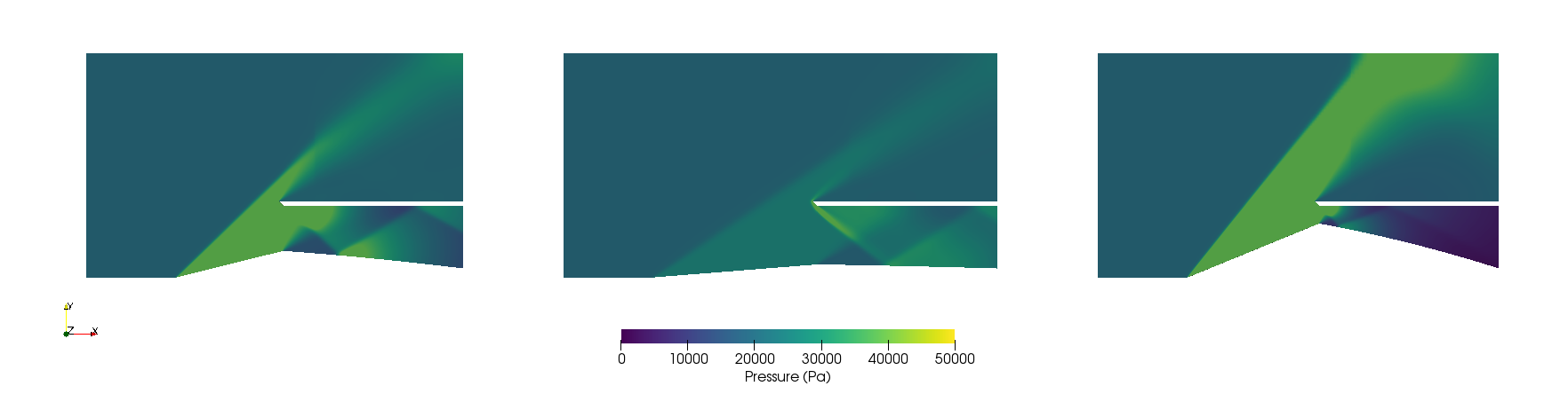
However, a sample from the last simulated generation looks like:
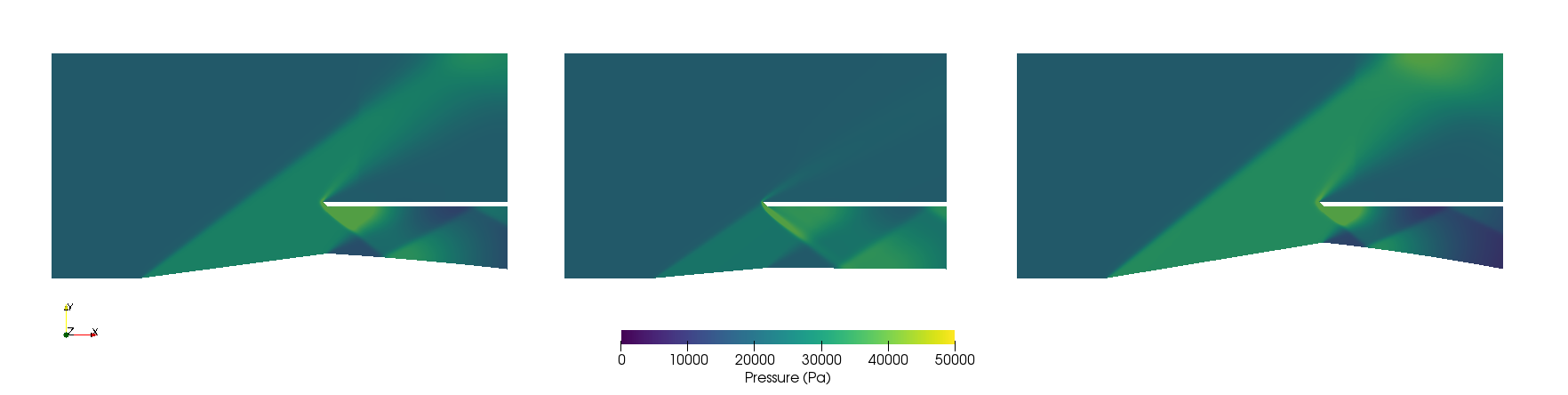
As it can be seen, the expected case where the shock wave meets the cowl is achieved, among other cases that exchange some pressure ratio for a higher Mach number on the outlet.
Airfoil shape optimization
Airfoils are the classical problem of optimization applied to CFD. However, it is usually solved with adjoint methods. In this project, a new approach has been used: geometrical optimization with genetic algorithms. Two different function space optimizations cases have been tested, but both depend on the same search space variables. Airfoils have been parametrized with a Joukowsky transform that depends on mu_x and mu_y as the coordinates of the circle in the Zeta plane. Although it may seem that a circle is fully defined with three parameters (x and y positions of the center and radius), the radius in this case must be fixed so the circle always intersects (-1,0) or (1,0), having two possible circles in the Zeta plane (and keeping the one that faces the freestream from left to right). Making the restriction that instead of having a variable radius, the shape obtained in the zeta plane will look like as an airfoil (more or less) and weird self-intersecting shapes will be avoided.
Before showing up the results of the two different optimizations, it is worth noticing that the only differences between the two are just one Python script used to include a different fitness computation (and its reference in the fitness.py). This shows the adaptability of the code.
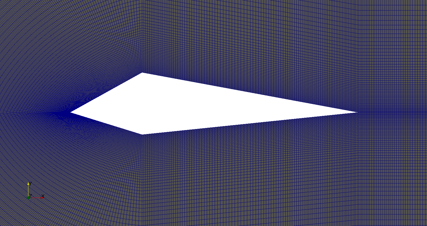
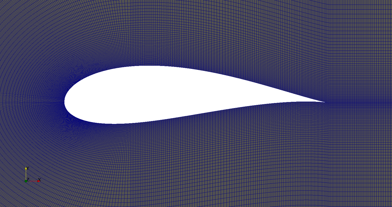
The mesh has been previously designed in 6 blocks that have a diamond-shaped airfoil in the center that is converted to an airfoil depending on the values of mu_x and mu_y of the Joukowsky transform by applying blockMesh to a file with the coordinates of the transformation:
 |
 |
Lift and drag
The first case, the two objective space functions that have been tried are the classical lift versus drag comparison. There is a trade-off between lift and drag in airfoils, as it can be seen in the majority of the polar diagrams. The results after the optimization process are:
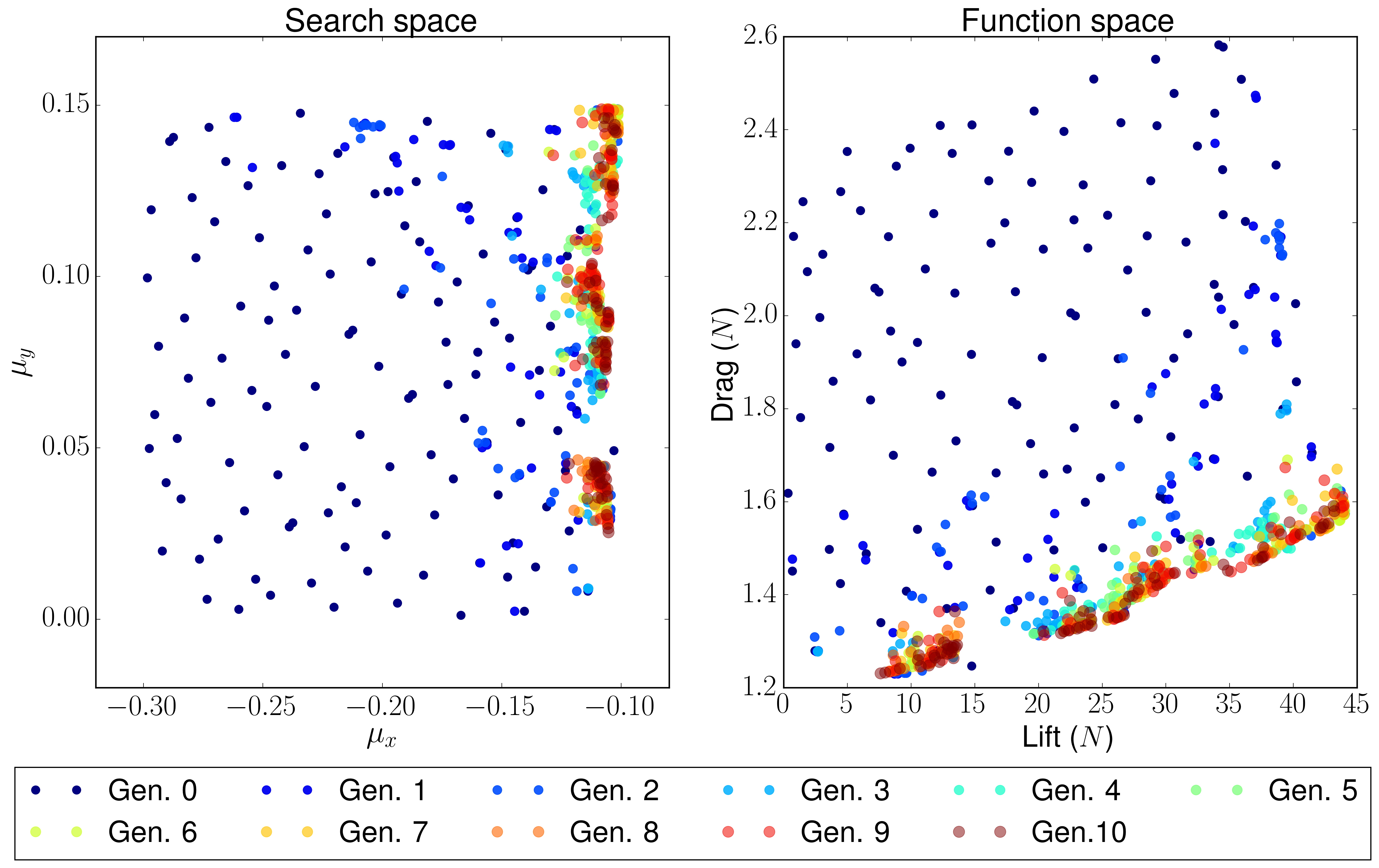
One sample of the first generation is:
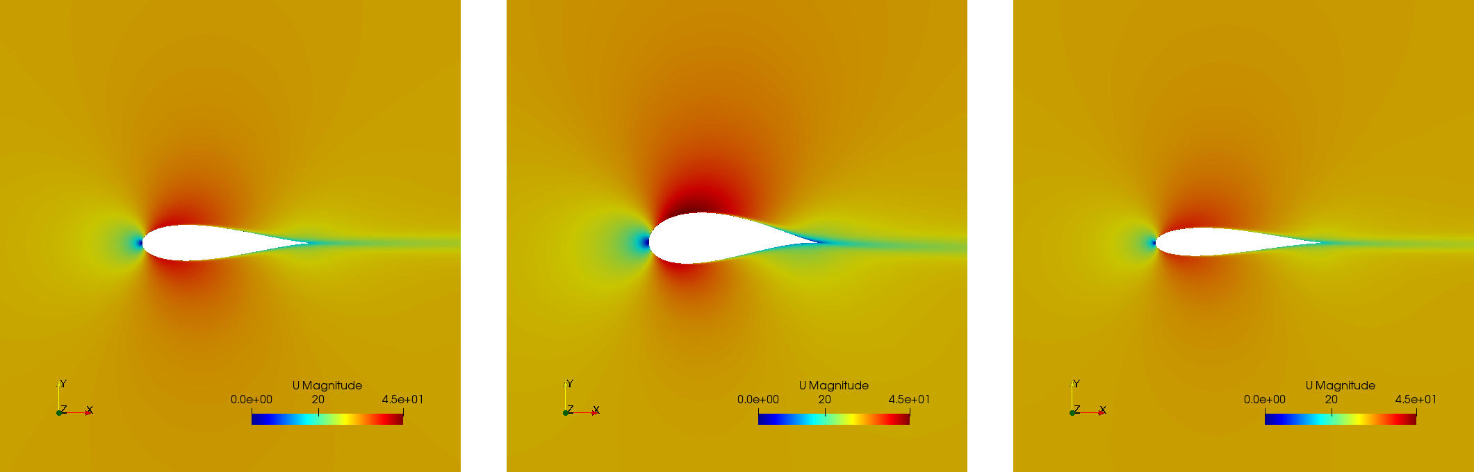
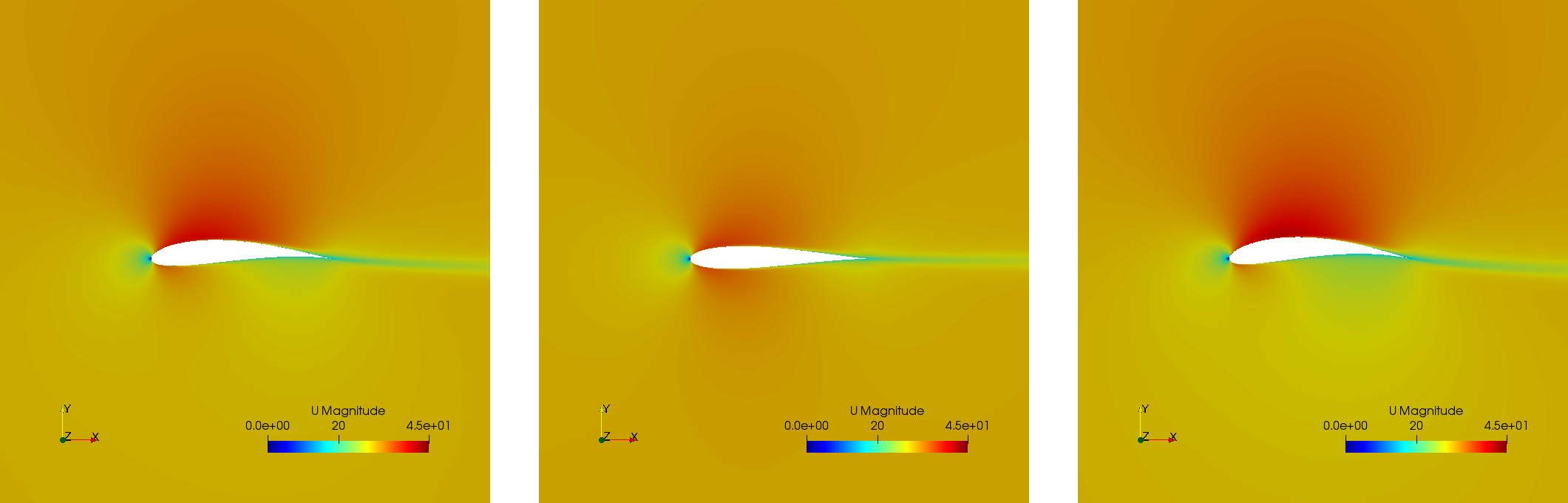
Three airfoils taken from the last generation show that the airfoils are thin and have a wide variety of curvatures:
Lift-to-drag ratio and area
The search space x and y axis are the same as before, but the distribution of the Pareto front is different. The function space has different objectives: Lift-to-drag ratio and area. Both are tried to be maximized:
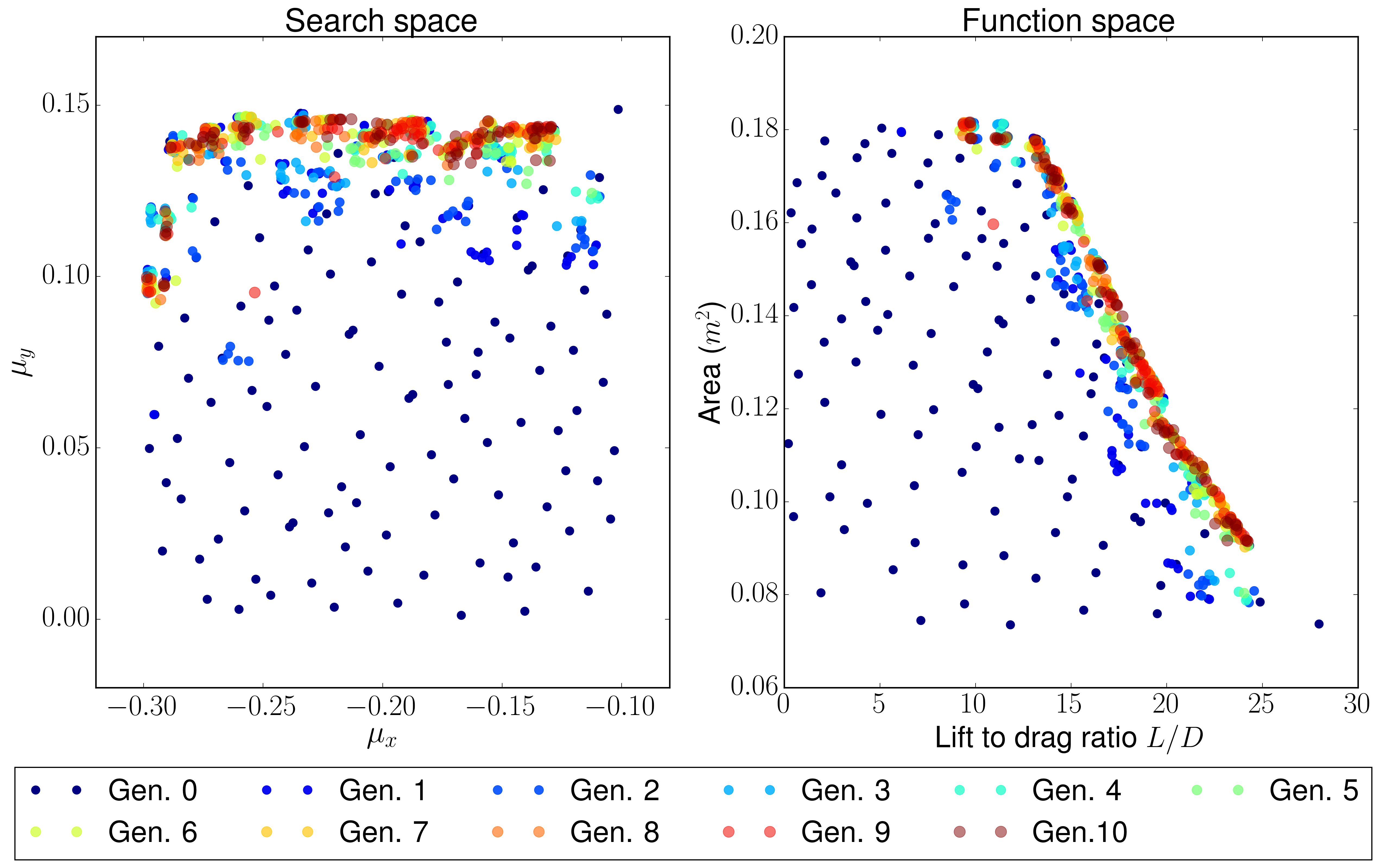
A sample of the first generation is the one shown in the image below (but the sample for the initial generation shown in the previous section would be also a valid sample because Sobol initialization was used, which is a quasi-random low discrepancy sequence that returns the same sampling points for both cases):

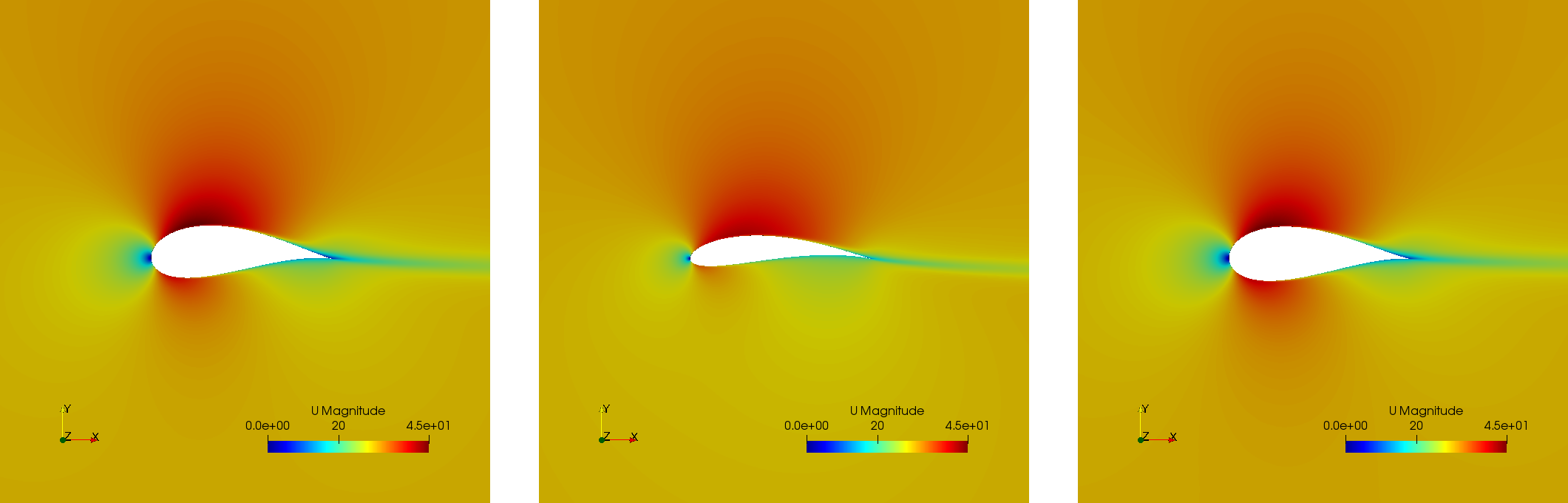
However, the results of this case are way different from the ones before. These have a larger inner area of the airfoil for most of the cases or a higher curvature:
Conclusions
The main objective of the project of coupling genetic algorithms with computer fluid dynamics cases has been fulfilled. The created scripts have been used for three different cases, proving that GA are a good approach to CFD but (at this thesis moment) only for 2D simple cases, given that each one of the optimization processes took ~20 hours and created roughly 50 Gb of data. Further developments should aim towards a higher convergence of the Pareto front to reduce both computational time and used space, so this method can be used for more complex cases or even 3D meshes.
FOLDER BY FOLDER
A more detailed view of the project will be presented here, explaining folder by folder the notebooks and Python scripts that are in the repository.
12-steps-CFD
This folder contains the 12 notebooks of the MOOC course that Professor Lorena Barba kindly created with some of her post-doc students and it is a great introduction to CFD via Python notebooks and easily understandable equations. So before using any bigger computer fluid dynamics suite (as OpenFOAM) a basic knowledge on how does it works is required to take the most out of it (and without making large mistakes).
airfoil-parametrization
Three different airfoil parametrization processes have been carried out, having one folder for each one.
airfoil
Notebook to read airfoil points from a data file (as the ones that can be downloaded from airfoiltools), sort and convert them to upper and lower surfaces. Some functions are included to give more detail to the available points, i.e., get 150 points from an airfoil with 50 points with spline interpolation (including also a grading in the x-axis to get the higher point density where desired).
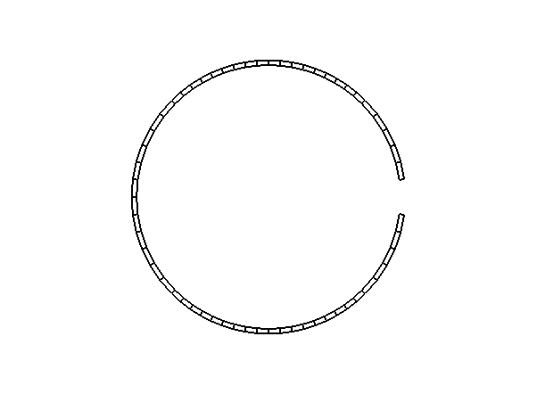
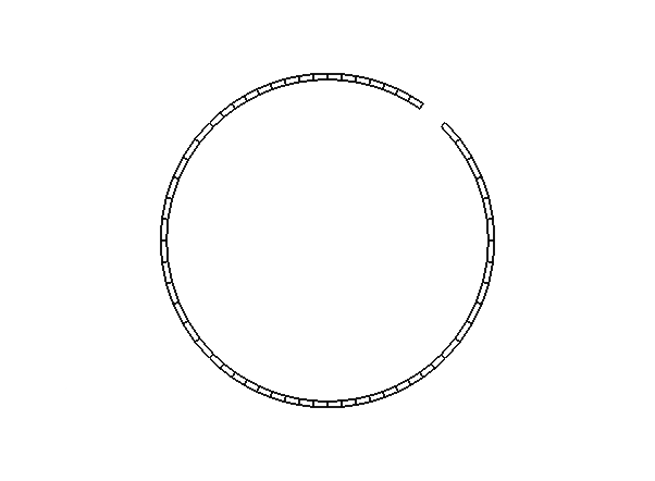
joukowsky
The Joukowsky transform has been coded in a detailed notebook for a circle defined with three parameters (position of the center and variable radius) and a circle defined only with the center (having a fixed radius so the circle always goes through points (1,0) and (-1,0), having shapes that look like airfoils). Joukowsky transformation with variable radius may create outputs like:
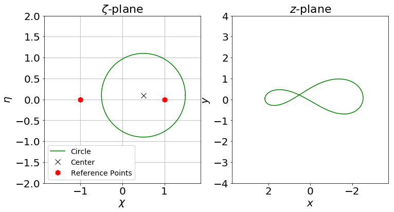
whereas the transformation with fixed radius give two possible airfoils:
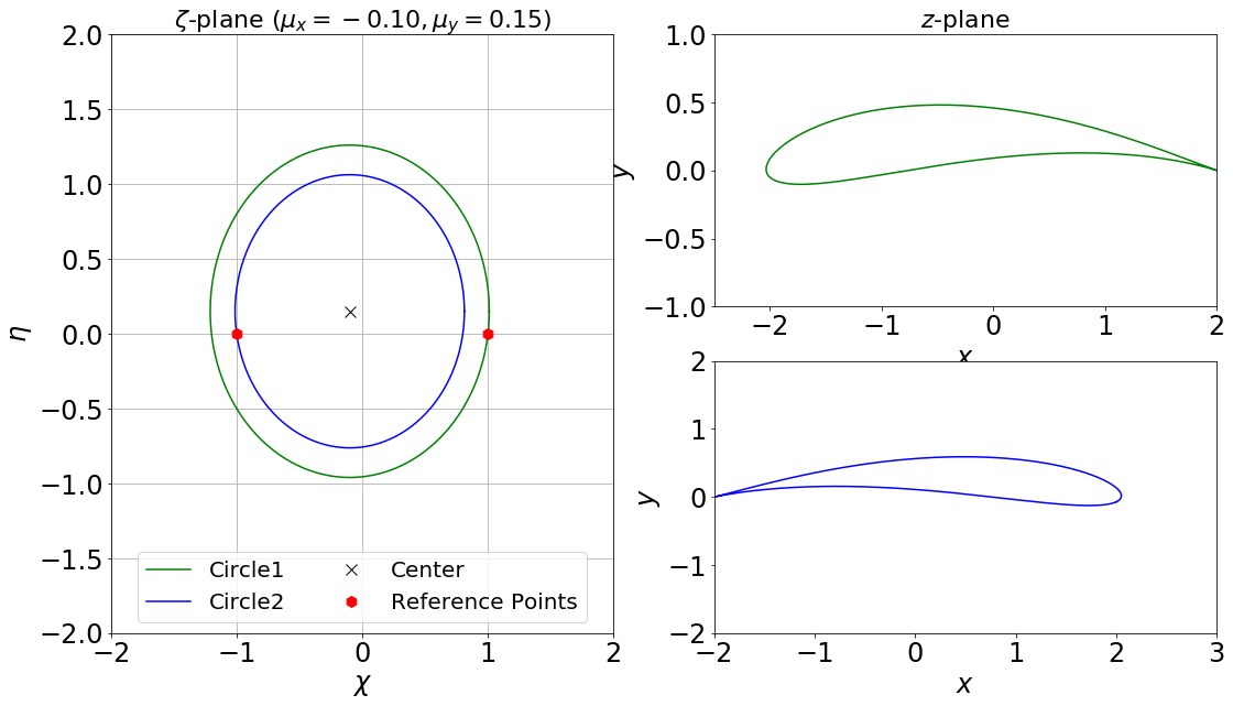
These codes have also been coded to be interactive, having sliders to change the center (and the radius when it is variable). The two .py files are interactive figures with sliders and to run them just execute python *.py in the terminal.
NACA4
The notebook has coded the required equations to compute a NACA 4-digit series airfoil, different grading tools to get points over certain range, interpolation of an airfoil over certain points (not very useful with airfoils whose equation is known though), and storage of the points in a .csv in a sorted way beginning from the trailing edge towards the leading edge over the upper surface and then back over the lower surface.
cases
This folder contains the initial folders for the fours cases introduced above (NSGA_cylinder, NSGA_diffuser, NSGA_joukowsky, NSGA_joukowskyCLCD). It also contains the results of these four simulations (these will differ due to the stochasticity of the algorithm) in the folder results/ .
templateCase
This folder contains the basic files, although they must be customized for the desired case.
evolution.py- Script with the NSGA-II implementation for (with a given population), compute the new one
fitness.py- Script to group the search space and function space of each generation in a text file, saving the values of all individual variables and functions (i.e., fitness)
initialization.py- Script to create the first initial population. There are three different initializations: random population, non-uniform low discrepancy sampling (Sobol sequences) or a uniform population. Although the initialization method should not be relevant (a number high enough of generations should yield the same results regardless of the initial generation), a careful decision must be taken, because CFD simulations take longer than a simple function evaluation (thus Sobol was chosen, using the same initial population for different fitness spaces)
problemSetup.py- This file contains the basics of the case such as the search space constraints or the number of individuals per generation
run- Bash script that will encompass the whole optimization process. This script is responsible for calling the different Python scripts, create the folders to store the data and advance in the generation count
runGen- Bash script to manage each generation: from the simulation to the generation of a new population. It begins with the distribution of the available resources, i.e., the number of processors (
procLim) for the individuals of the generation (nProc), so all the (desired) processors are running at the same time. It includes the decomposition of the case, running the OpenFOAM application with openMPI and the reconstruction of the case (though not essential for all analysis). This is achieved by managing the process identifies (PID) number of the different simulation, so once a simulation has finished, another one begins. Postprocessing and fitness evaluation is also included in this bash script, closing with the calling toevolution.pyto create a new population.
Some of the things (amongst others) that are required to be changed before running the optimization for a custom case are listed below:
- Include the
baseCasefolder - Create a script to include the different variables in the case (whether in a blockMesh fashion or in the boundary conditions)
- Code commands in
runGenif required: such asblockMeshfor the pre-processing part of the simulation or some fitness evaluation commands (e.g.pvbatch). - Change the name of the files according to the variables (only if desired, not required)
- Modify the fitness script
There are four working cases in the repository with all required files to complete the optimization. These may serve as further reference.
cavity-mesh
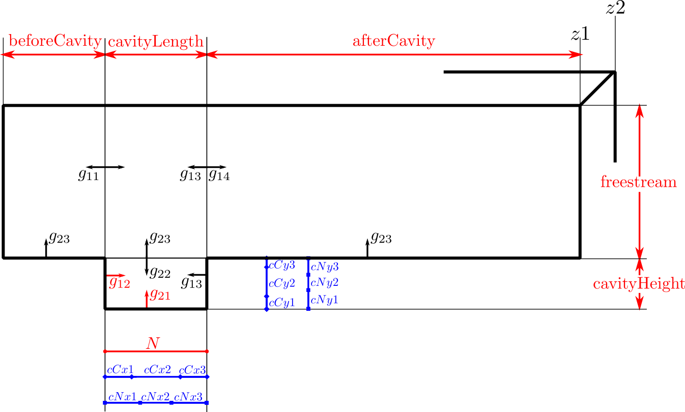
Mesh generator of a cavity inside a freestream flow with a high level of customization but keeping in mind one objective: maintain the aspect ratio with a value of 1 in the vast majority of the cells that are far from the boundary layer. Basic inputs are the dimensions of the case, having three horizontal dimensions (freestream beforeCavity -bC-, horizontal cavityLength -cL-, freestream afterCavity -aC-) and two vertical ones (cavityHeight -cH- and freestream height -f-), number of horizontal cells in the cavity (N) and grading (boundary layer expansion ratio factor) of the most-left wall and lower wall of the cavity (g12 and g21). There are additional inputs to the case that may also be varied: z-direction components (z1 and z2) and percentage of the chord and cells for each percentage in the cavity block (cCx1, cCx2, cCx3, cCy1, cCy2, cCy3, cNx1, cNx2, cNx3, cNy1, cNy2, cNy3). Custom gradings for all the other walls are also additional inputs, but if not specified they will be computed automatically depending on the ones fixed for the other directions.
The inputs are shown in the next figure, having red for the mandatory inputs, blue for the additional ones and black for the ones that will be computed (unless otherwise specified):
The computed values are sketched in the figure below:
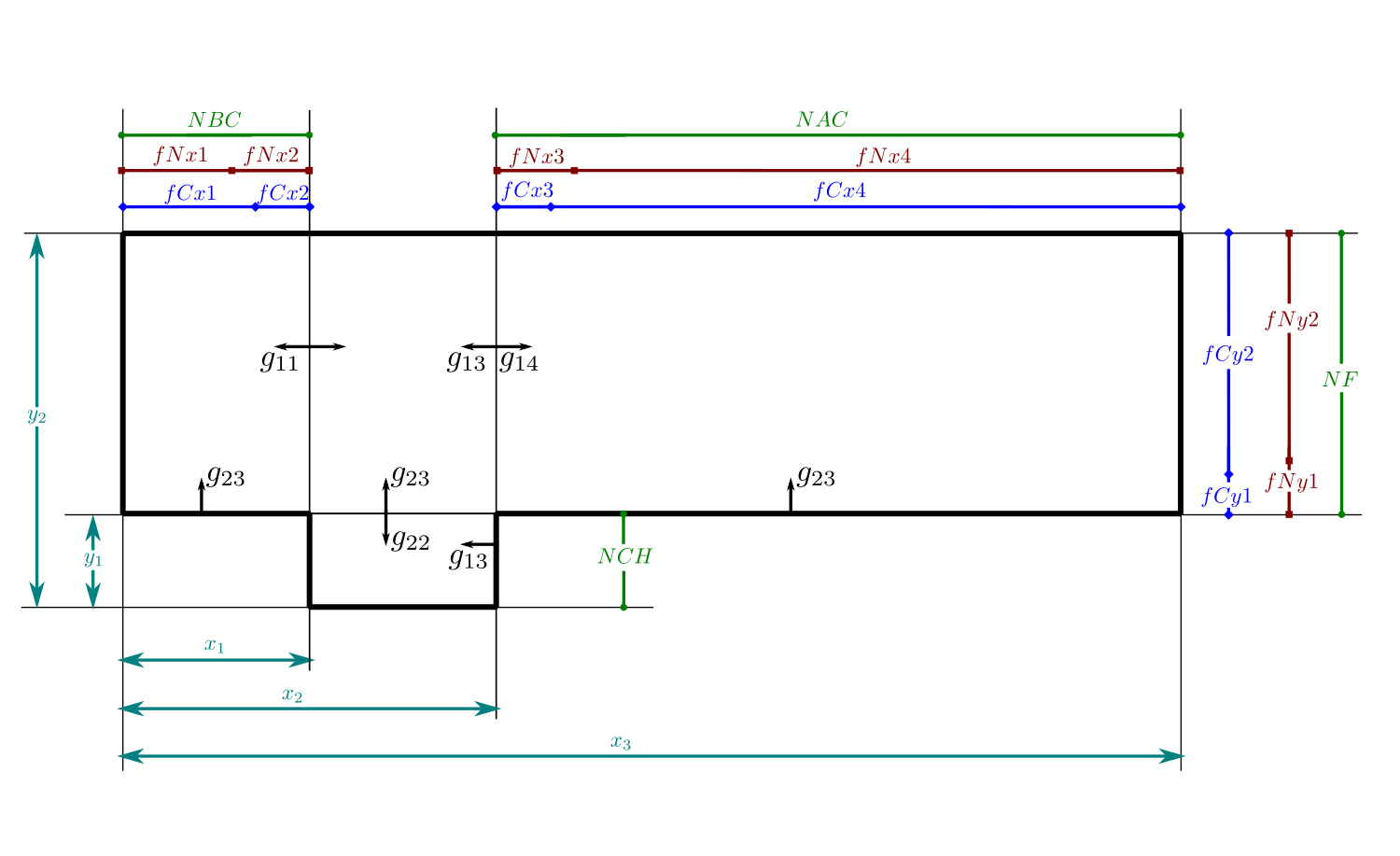
First of all, the dimensions x1, x2, x3, y1, and y2 are computed with the specified individual dimensions. There are some values in the previous sketch that are straightforward to compute, having that the different divisions of each block are computed by:
The number of cells for each dimension is computed so the greatest part of all blocks are squared cells with aspect ratio 1:1. To make that, the distance in the horizontal and vertical dimension of every cell are equaled and solved to get the number of cells in each direction. Keep in mind that total length times the length percentage divided by the total number of cells and by the percentage of cells will give the size of the cell.
- Solving for a cavity cell dimensions to obtain the number of cells in the cavity height:
- Freestream right-above-the-cavity cell to determine the number of cells in the freestream:
- Freestream before-the-cavity cell to obtain cells in the horizontal before-the-cavity length:
- Freestream after-the-cavity cell to obtain cells in the horizontal after-the-cavity length:
All the number of cell computations were rounded to the nearest integer to avoid decimal number of cells. Once the number of cells of each block has been computed, it is important to assign the percentage of cells for each block subdivision:
Finally, the different boundary layer inflations are computed by:
unless otherwise specified.
It can be seen in the next figure how a cavity mesh is obtained from some values. It is worth noticing that the freestream and a considerable section of the cavity is made of squared cells:
This folder is in this repository because cavity vortex shedding was another case which seemed interesting to control with genetic algorithms. However, the implementation was not possible due to time constraints.
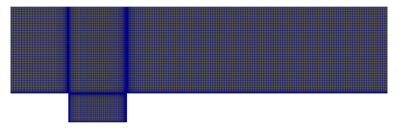
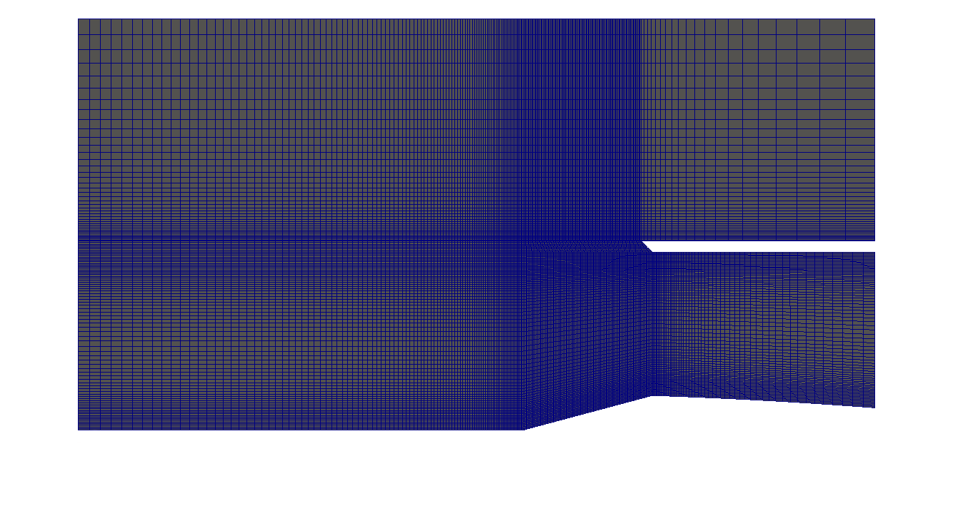
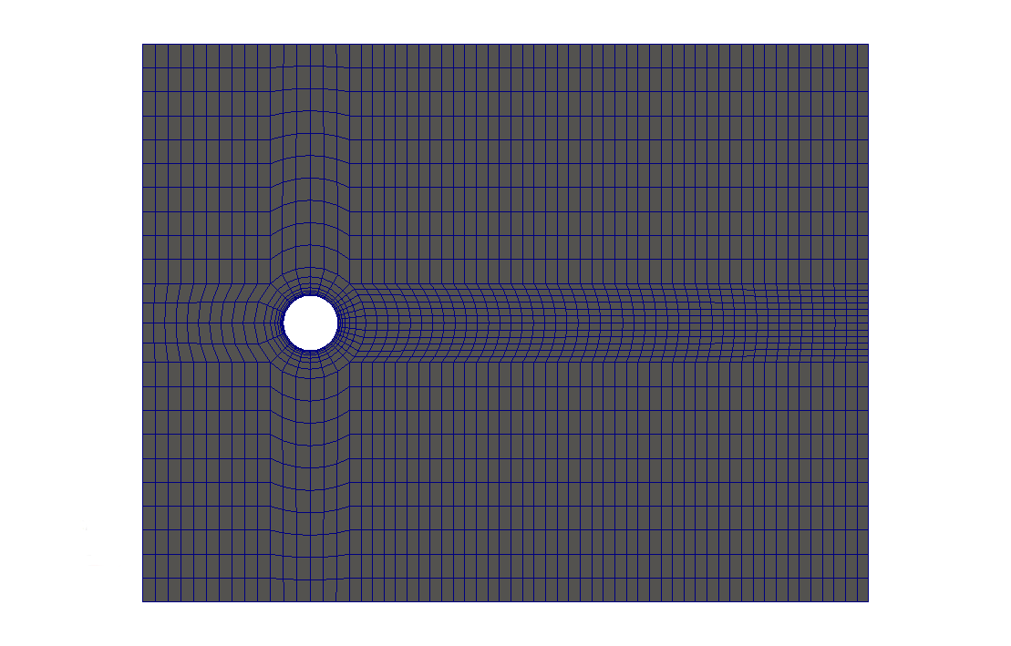
cylinder-mesh
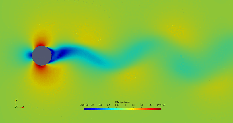
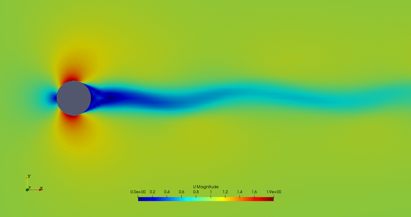
The first thing to notice in this folder is a mp4 video that shows forced vortex shedding with a boundary condition perturbation. Pressure and velocity_magnitude are represented in the left view while the white line values are represented in the right plot. Moreover, there are two folders that will be described now.
mesh-convergence
In the process of doing a mesh convergence, different mesh refinements were tried. However, and given the lack of validation values, it was a little hard to perform mesh convergence, because as it can be seen in the third column of cylinderMeshConv, the most refined the case, the stronger the vortex (which is obviously related to the cell size). The different meshes are also stored in the cases folder, the extracted data after the simulation of the mesh is stored in the data folder and it is analyzed with the notebook in the root of this folder.
mesh-flowControl
After mesh convergence, three meshes were created with different combinations of the location of the membrane, having a rear position (first column is a coarse mesh and the center column is a finer one) and a position right in the flow detachment point (third column) where membranes are usually located:
 |
 |
 |
Further developments should locate the flow inlet-outlet in a custom angle with a redefined mesh (these ones are too constrained and no modifications are possible).
diffuser-mesh
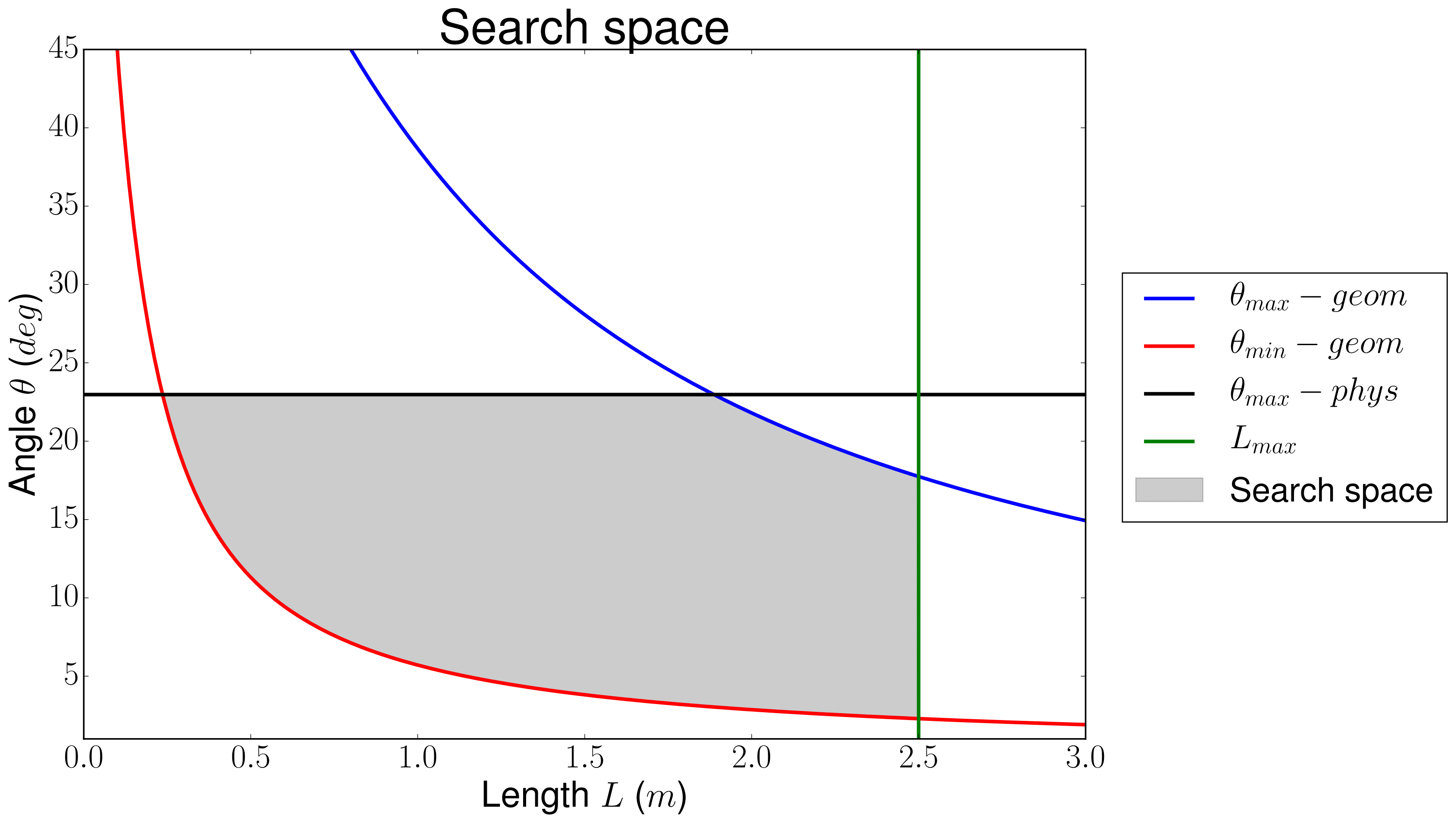
The mesh for the diffuser case is created with a Python script executed as python3 blockMeshGenerator.py L theta folderNum. This will create a ready-to-simulation folder (copy of the baseCase folder) with a mesh with the desired parameters for the length and angles of the inlet.
In this folder is also included the constrained search space for this case. There are 4 different constraints:
- Blue line: there is a geometrical constraint given that the angle cannot be as large as the 0.8-meter distance of the diffuser exit length (measured from the axis). Therefore, for each length, there is a maximum possible angle where the inlet of the diffuser meets the cowl of the engine.
- Red line: as before, there is a lower bound for the angle, given that minimum increase in ''height'' from the axis is 0.1 meters. Again, for each length, there is an angle where the inlet of the diffuser will be tangent to the outlet of the diffuser (having a diffuser with parallel surfaces).
- Green line: is a geometrical constraint that refers to a maximum length of the diffuser, i.e., it limits the diffuser length to avoid inlets of more than 2.5 meters (which already is a long enough case).
- Black line: this is the physical constraint to the angle variable, given that attached oblique shockwaves (which are more stable than the detached ones) behave according to the
theta-beta-Machequation (from compressible flow theory) and there is an upper limit in the angle that a shock wave may suffer before detaching it from the leading edge of the step that it encounters.
These constraints are coded up in the notebook, obtaining a space with the next shape:
mesh-generation
In this folder, there are different Jupyter notebooks that go step by step in the process of generating different meshes for simulation with OpenFOAM. All notebooks are functional and modify the different meshes (saving in the respective folder) directly from the notebook itself (except the joukowskyMesh folder which includes a Python script for that purpose).
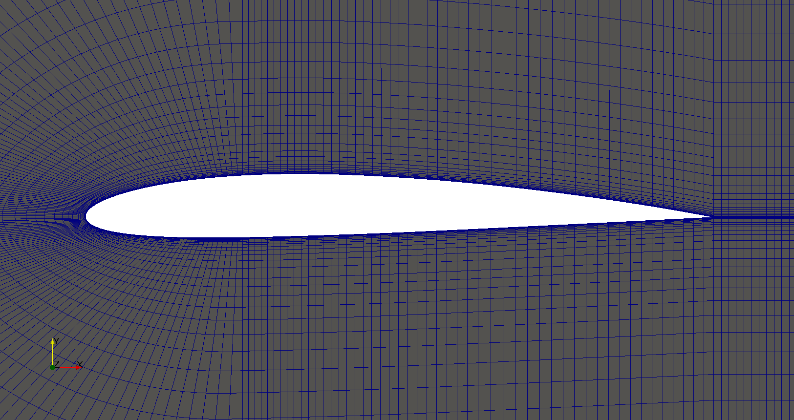
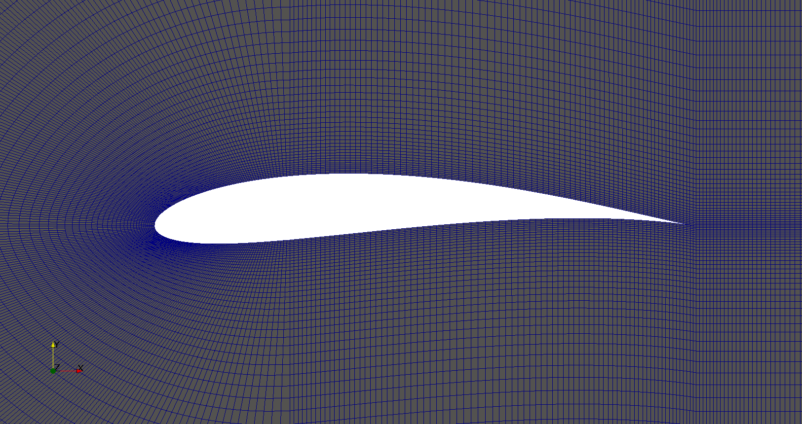
extMesh
This mesh generation includes different parameters for a customized mesh: from the number of cells and the expansion ratio to NACA profile selection. It creates the required mesh for a simulation of the flow outside an airfoil, as shown below:
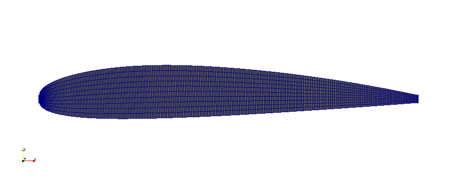
int
This case was done before the external mesh generator so it includes the different details. It creates a mesh in the inner part of the airfoil (what may be useful for structural calculations), as shown in the image below:
joukowskyMesh
A .py script includes all necessary to generate a Joukowsky airfoil with the x and y coordinates of the center as inputs in the command line (ensure that it is a valid center, whose circumference goes through the control points). Case folder will include the mesh for the simulation.
This script was afterward modified to store the airfoil in a folder with a certain name, in order to apply it to the optimization cases. In the figure below, a sample case may be seen.
str_uns
Given that flow control in the cylinder with the membrane in the rear part of the cylinder had some problems concerning mixing of the flow, an ''unstructured'' mesh was created from the blockMesh of the cylinder case by slightly perturbing the different nodes (as shown below, having the structured mesh in the left and the unstructured one on the right):
 |
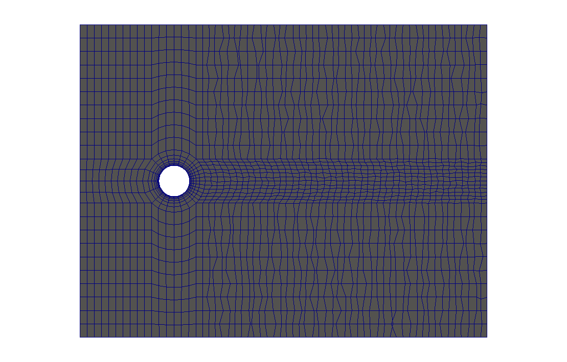 |
This idea was deprecated given that the results of the simulations were not conclusive and no special mixing or diffusion was observed on the unstructured mesh.
openFoam-case
The first approach to genetic algorithm implementation was done entirely with Python scripts (instead of with bash scripts). The classical pitzdaily simulation was used, with a simplified mesh for quicker runs and different velocities to test the use of different variables in the case.
However, it ended up being a little messy because calling subprocesses from Python scripts and executing different cases was hard to do in a neat way.
The initial folder layout was:
case/
├── baseCase/
│   ├── 0/
│   ├── constant/
│   └── system/
└── run/
    ├── allRun.py
    └── plotting.py
The final folder structure will look like:
case/
 ├── baseCase/
 │   ├── 0/
 │   ├── constant/
 │   └── system/
 └── run/
     ├── generation0/
         │   ├── ind0/
         │   │   ├── sim/
         │   │   │   ├── 0/
         │   │   │   ├── ...
         │   │   │   ├── constant/
         │   │   │   └── system/
         │   │   ├── continuity.png
         │   │   ├── forces.png
         │   │   └── residuals.png
         │   ├── ...
         │   └── ind$N/
     ├── ...
     ├── generation$gL/
     ├── allRun.py
     └── plotting.py
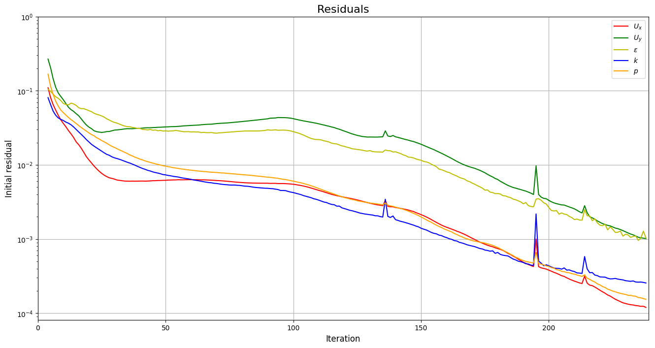
Although the implementation with Python scripts was not used, the scripts folder includes some useful progress bars (both for command line interface and GUI) and the plotting.py script allows to create plots of the output of different OpenFOAM solvers, obtaining figures with the residuals (and also convergence and forces):
optimization
The optimization folder includes different subfolders as well as different notebooks listed below:
NSGA_II.ipynb: this notebook includes all the NSGA-II implementation step-by-step, including figures to show how every step of the intricate process of generating a new population really works. It also applies the algorithm to one function and saves the results (so it can be used as a NSGA-II script in the figures and others are commented).basicsMachineLearning.ipynb: at the beginning of the thesis, different machine learning concepts sounded strange, so the basic implementation of an artificial neural network with backpropagation and a simple genetic algorithm to decrypt codes were coded up.comparison.ipynb: when comparing random search, general-purpose genetic algorithm, and NSGA-II, this script first runs each method independently and then creates histograms for different test functions to see how well does each search method behave. Also, a comparison between the number of generation and the number of individuals was used to determine the best combination (given that these runs took a long time, data is saved and only loading it is required).multiobjective_MC_GA.ipynb: before getting to know NSGA-II, an implementation of a genetic algorithm for multiobjective optimization was carried on my own, in order to learn what was useful and required for a GA to achieve a good performance and get a precise solution in the Pareto front.singleObjective_MC_function_optimization.ipynb: a basic random search (a.k.a. Monte Carlo method) was implemented for single objective functions. Tests on convergence and error were done. An 'optimized' Monte Carlo method (that involved a little of evolution by moving the points towards points within a Gaussian distribution) was used, and although it improved the behavior of the plain random search, it was not enough.
NSGAIIpics
As the name states, it includes all kind of pictures of the NSGA-II, in order to include them in either the presentation or the report, as well as the first (funny) run of the algorithm.
Pareto_fronts
Data from a machine learning framework with the true solution of different Pareto fronts.
comparisonData
Data extracted after running the comparison.ipynb notebook, and given that it took so long, results were saved in this folder.
figures
Figures of the comparison.ipynb notebook, showing the results of the data.
vortex-generation
After obtaining vortex shedding with a perturbation in the inlet boundary condition, data of two streamlines (one above and one below the cylinder) was extracted with the Python script designed for Paraview. It was afterward analyzed with the vortexGeneration_analysis notebook that also included the generation of different boundary condition for the flow control membrane (according to the frequency of the vortex shedding).
That's all folks!
REFERENCES
| [1] | Sóbester, András, and Alexander IJ Forrester. Aircraft aerodynamic design: geometry and optimization. John Wiley & Sons, 2014. |
| [2] | (1, 2) Deb, Kalyanmoy, et al. "A fast and elitist multiobjective genetic algorithm: NSGA-II." IEEE transactions on evolutionary computation 6.2 (2002): 182-197. |
| [3] | Townsend, A. A. R. "Genetic Algorithm-A Tutorial." Av.: https://pdfs.semanticscholar.org/eccb/f6523d2d29a5f6dbed9d7a0210e5ded49b96.pdf (2003). |
| [4] | Schaffer, J. David. "Multiple objective optimization with vector evaluated genetic algorithms." Proceedings of the First International Conference on Genetic Algorithms and Their Applications, 1985. Lawrence Erlbaum Associates. Inc., Publishers, 1985. |
| [5] | Fonseca, Carlos M., and Peter J. Fleming. "Multiobjective genetic algorithms." Genetic algorithms for control systems engineering, IEE colloquium on. IET, 1993. |
| [6] | Yen, Gary G., and Haiming Lu. "Dynamic multiobjective evolutionary algorithm: adaptive cell-based rank and density estimation." IEEE Transactions on Evolutionary Computation 7.3 (2003): 253-274. |


