I wish to plot a forest plot using this package with the text labels in the first column being one colour (or a selection of colours), and the remaining columns remaining black. The following MWE generates a plot of the type I wish to modify:

library(forestplot)

cohort <- data.frame(Age = c(43, 39, 34, 55, 70, 59, 44, 83, 76, 44, 
                             75, 60, 62, 50, 44, 40, 41, 42, 37, 35, 55, 46), 
                     Group = structure(c(1L, 1L, 1L, 1L, 1L, 1L, 1L, 1L, 1L, 1L, 
                                         1L, 1L, 1L, 1L, 1L, 2L, 2L, 2L, 2L, 2L, 2L, 2L), levels = c("1","2"), class = "factor"))

age.lm <- lm(Age ~ Group, data = cohort)
age.data <- summary(age.lm)$coefficients[2,]
age.data <- rbind(c(0,0,0,1,"Group 1", "n=15"),
                  c(age.data[1], age.data[1]-age.data[2]*1.95, 
                  age.data[1]+age.data[2]*1.95, age.data[4], "Group 2", "n=7"))
colnames(age.data) <- c("mean","lower","upper","p-val","labeltext","numbers")
age.data <- data.frame(age.data)

age.data$mean <- as.numeric(age.data$mean)
age.data$lower <- as.numeric(age.data$lower)
age.data$upper <- as.numeric(age.data$upper)

age.plot <- forestplot(age.data,
           labeltext = c(labeltext,numbers),
           boxsize = 0.1,
           xlog = FALSE,
           clip=c(-20,20),
           xticks=c(-20,-10,0,10,20),
           txt_gp = fpTxtGp(ticks=gpar(cex=1)),
           align=c("l","c","l"))

This generates a monochrome plot, but I want the labels for the groups to be different colours like (mockup):

This is currently not possible using fpColors(text=...), as this colours the text in all columns on each row.

(I am aware it can be done in post-processing, but would prefer a programmatic solution in the script generating this plot)

Is it possible to add a vertical line positioned at x=1 and not x=0 to a forest plot created by 'forestplot' function?

I have tried several different methods to change the font size of the xticks and xlab, such as cex.axis, cex.lab, cex, pch, fontsize, etc. But all of them didn't work. Could you give me some suggestions to change them? Thanks.

Dear Max,
I have met an isuue when using xlog=TRUE. I want to draw a grid line of 0.5. But the grid line is actullay positioned in e^0.5.

row_names <- list(list("test = 1", expression(test >= 2)))
test_data <- data.frame(coef=c(0.3, 5.24),
                        low=c(0.1, 3.78),
                        high=c(1.1, 8.55))
forestplot(row_names,
           test_data$coef,
           test_data$low,
           test_data$high,
           zero = 1,
           grid=structure(c(0.5), gp=gpar(color="steelblue", lty=2)),
           cex = 2,
           lineheight = "auto",
           xlog=TRUE,
           xticks=c(0.1,1,10))

I also tried to enter -0.69, which equals to log(0.5,e). But it report an error.

> row_names <- list(list("test = 1", expression(test >= 2)))
> test_data <- data.frame(coef=c(0.3, 5.24),
+                         low=c(0.1, 3.78),
+                         high=c(1.1, 8.55))
> forestplot(row_names,
+            test_data$coef,
+            test_data$low,
+            test_data$high,
+            zero = 1,
+            grid=structure(c(-0.5), gp=gpar(color="steelblue", lty=2)),
+            cex = 2,
+            lineheight = "auto",
+            xlog=TRUE,
+            xticks=c(0.1,1,10))
Error in forestplot.default(row_names, test_data$coef, test_data$low,  : 
  All argument values (mean, lower, upper, zero, grid and clip) should be provided as exponentials when using the log scale. This is an intentional break with the original forestplot function in order to simplify other arguments such as ticks, clips, and more.

Actually, this issue is exactly the same as #14 and #10 which had been closed.
In #14, the author solved the issue through updating packages from github. I have tried to update my packages to version 1.7.2, but it doesn't work. In #10, the author didn't state his solution.

I'm really looking forward for your advise.

Hi,

When I plot the forestplot from dataframe containing only one row, the error happened:

tt <- data.frame(
  mean = 3, upper = 4, lower = 2, P = 0.01, gene = "XX"
)
tt |>
  forestplot(labeltext = c(gene,P),
             xlog = TRUE,
             xlab = "OR",boxsize = 0.25) |>
  fp_set_style(box = "royalblue",
               line = "darkblue",
               summary = "royalblue") |> 
  fp_add_header(gene = c("gene"),
                P = c("P")) |>
  fp_set_zebra_style("#EFEFEF")

Error in prepLabelText(labeltext = coreData$labeltext, nr = nrow(coreData$estimates)) : 
  You have provided 1 rows in your mean arguement while the labels have 2 rows

add another row, it can plot:

tt <- bind_rows(tt,tt)
tt |>
  forestplot(labeltext = c(gene,P),
             xlog = TRUE,
             xlab = "OR",boxsize = 0.25) |>
  fp_set_style(box = "royalblue",
               line = "darkblue",
               summary = "royalblue") |> 
  fp_add_header(gene = c("gene"),
                P = c("P")) |>
  fp_set_zebra_style("#EFEFEF")

Thanks a bunch for making such a useful package! I'm having an issue whereby in the function forestplot, when xlog = FALSE, the lower bound specified by the clip argument doesn't appear to have any effect.

Below's an example that replicates the behaviour (taken in large part from the vignette: https://cran.r-project.org/web/packages/forestplot/vignettes/forestplot.html). You'll see for the first forestplot where xlog = TRUE, everything appears to work as expected. But for the second, where xlog = FALSE, the clipping doesn't seem to be having the impact it should.

library(forestplot)

# Cochrane data from the 'rmeta'-package
cochrane_from_rmeta <- 
  structure(list(
    mean  = c(NA, NA, 0.578, 0.165, 0.246, 0.700, 0.348, 0.139, 1.017, NA, 0.531), 
    lower = c(NA, NA, 0.372, 0.018, 0.072, 0.333, 0.083, 0.016, 0.365, NA, 0.386),
    upper = c(NA, NA, 0.898, 1.517, 0.833, 1.474, 1.455, 1.209, 2.831, NA, 0.731)),
    .Names = c("mean", "lower", "upper"), 
    row.names = c(NA, -11L), 
    class = "data.frame")

tabletext <- cbind(
  c("", "Study", "Auckland", "Block", 
    "Doran", "Gamsu", "Morrison", "Papageorgiou", 
    "Tauesch", NA, "Summary"),
  c("Deaths", "(steroid)", "36", "1", 
    "4", "14", "3", "1", 
    "8", NA, NA),
  c("Deaths", "(placebo)", "60", "5", 
    "11", "20", "7", "7", 
    "10", NA, NA),
  c("", "OR", "0.58", "0.16", 
    "0.25", "0.70", "0.35", "0.14", 
    "1.02", NA, "0.53"))

forestplot(tabletext, 
           cochrane_from_rmeta,
           clip = c(0.2, 2.5), 
           xlog = TRUE)

forestplot(tabletext, 
           cochrane_from_rmeta,
           clip = c(0.2, 2.5), 
           xlog = FALSE)

Thank you for this package. I'm finding it very useful.

I'm having issues with lineheight and line.margin. They do not appear to be functional and lineheight is auto regardless of my input.

Please see below example. Please let me know if I have made an obvious error!

author_year <- c("A 2023" , "B 2020" , "C 2003")
analysis <- c("unadj" , "adj" , "adj")
int_event <- c(200 , 150 , 100)
int_total <- c(400 , 400 , 300)
cont_events <- c(50 , 150 , 100)
cont_total <- c(105 , 300 , 200)
or <- c(1.5 , 1.1 , 1.3)
lowerci <- c(1.1 , 0.7 , 0.9)
upperci <- c(2.0 , 1.9 , 1.6)

df <- data.frame(author_year , analysis , int_event , int_total , cont_events , cont_total , or , lowerci , upperci)
df

df %>%
forestplot(labeltext = c(author_year , analysis , int_event , int_total , cont_events , cont_total) ,
mean = or ,
lower = lowerci ,
upper = upperci ,
xlog = TRUE ,
lineheight = unit(0.1 , "cm")) %>%
fp_add_header(author_year = c("", "Study") ,
analysis = c("", "Analysis") ,
int_event = c("Int" , "events") ,
int_total = c("" , "total") ,
cont_events = c("Cont" , "events"),
cont_total = c("", "total")) %>%
fp_set_zebra_style("#EFEFEF")

Is it possible to add colors to ticks and xlabs? It works perfectly for labels but I can't make it work for xticks or xlabs...

txt_gp = fpTxtGp(label = list(gpar(fontfamily = "HersheyScript"),
gpar(fontfamily = "",
col = "#660000")),
xlab = gpar(fontface = "bold", cex = 1.5, col = "#660000"))
ticks = gpar(fontface = "bold", col = "blue", cex=1))

I found an error using grouped forestplots when extra columns are used beyond the basic labeltext variable next to the forestplot. In the vignette the grouped examples don't use the "labeltext" parameter call.

When modifying the example in the vignette to add the estimate:

library(forestplot)
data(dfHRQoL)


dfHRQoL <-dfHRQoL |>
  mutate(est = sprintf("%.2f", mean), .after = labeltext)

dfHRQoL |>
  group_by(group) |>
  forestplot(labeltext = c(labeltext, est),
             clip = c(-.1, 0.075),
             ci.vertices = TRUE,
             ci.vertices.height = 0.05,
             boxsize = .1,
             xlab = "EQ-5D index") |> 
  fp_add_lines("steelblue") |> 
  fp_add_header(Variable="Variable", est = expression(beta)) |> 
  fp_set_style(box = c("blue", "darkred") |> lapply(function(x) gpar(fill = x, col = "#555555")),
               default = gpar(vertices = TRUE))

Gives this error:

Error in forestplot.grouped_df(group_by(dfHRQoL, group), labeltext = c(labeltext, :
There are seem be invalid the labels: 85 vs 65 years > -0.04
appear in the wrong position.

I am struggling to show vertical reference lines in my forest plot.
In the very last example in the vignette (as of 2022-10-09), it is shown how to modify grid lines: "You can easily customize both what grid lines to use and what type they should be by adding the gpar object to a vector". However, in the plot that is generated by the example there are no grid lines at the expected positions.
Also, I am somewhat confused about the syntax, since there now seems to be an argument "grid" in the fp_set_style to provide a gpar for the grid, but the aforementioned example shows a different way to provide the gpar directly in the "grid" argument of "forestplot".

Any help or explanation would be highly appreciated.

I would like to combine 2 plots, 1 row with panels (2 separate forest plots) and add panel labels (letters a & b)

Is there an option similar to grid.arrange/par(mfrow=c(1,2)) that can be used?

par(mfrow=c(1,2)) seems not to work

There is an issue when editing the box colors to all be different.

When adding to forestplot(), col = fpColors(box = c("black", "blue", "red")) it will make all the boxes black.

In fact I found that it will always make all the colors whatever the first entry in the color vector is, so if instead I made it col = fpColors(box = c("red", "blue", "black")) then they would all show up as red.

Bug description

When labeltext is a list, graph.pos cannot be set to any value above 2. That bug is due to incorrect calculation of the number of columns of the list.
The following code illustrate this problem:

author=expression(paste("Smith ", italic("et al")))
pseudomat=list(Author=list(author, author), Year=list(2002,2005), N=list(50,75), Weight=list(0.40,0.60))
forestplot(labeltext = pseudomat, mean=1:2, lower=0:1, upper=4:5, graph.pos=4)

Expected behavior: display three data columns (Author, Year, N), then, the forest plot, than a fourth data column (Weight).
Observed behavior: the following error is raised: "Error in forestplot.default(labeltext = pseudomat, mean = 1:2, lower = 0:1, :
The graph position must be between 1 and 2. You have provided the value '4'."

Current workaround

Sets the class of pseudomat to "data.frame" in order to override the behavior of ncol().

author=expression(paste("Smith ", italic("et al")))
pseudomat=list(Author=list(author, author), Year=list(2002,2005), N=list(50,75), Weight=list(0.40,0.60))
class(pseudomat)="data.frame" # workaround (ugly hack)
forestplot(labeltext = pseudomat, mean=1:2, lower=0:1, upper=4:5, graph.pos=4)

That hack is horrendous. The pseudomat object becomes a corrupted data.frame object, hybrid between a list of list and a real data.frame, tricking forestplot for its ncol() calculation.

Bug fix

This bug can be found on line 442 to 447 of the forestplot.R file. The code checks that the graph.pos is in the correct range, but uses NCOL(labeltext) rather than nc as the number of columns.

See pull request 81dc455

Test environment

Package: forestplot
Version: 1.9
Maintainer: Max Gordon [email protected]
Built: R 4.1.0; ; 2020-07-09 04:36:23 UTC; windows

R Version:
platform = x86_64-w64-mingw32
arch = x86_64
os = mingw32
system = x86_64, mingw32
status = Under development (unstable)
major = 4
minor = 1.0
year = 2020
month = 07
day = 11
svn rev = 78812
language = R
version.string = R Under development (unstable) (2020-07-11 r78812)
nickname = Unsuffered Consequences

Windows 10 x64 (build 17134)

Locale:
LC_COLLATE=French_France.1252;LC_CTYPE=French_France.1252;LC_MONETARY=French_France.1252;LC_NUMERIC=C;LC_TIME=French_France.1252

Search Path:
.GlobalEnv, package:forestplot, package:checkmate, package:magrittr, package:grid, package:stats, package:graphics,
package:grDevices, package:utils, package:datasets, package:methods, Autoloads, package:base

Current feature and limitation

The col parameter of the forestplot function can be set to a fpColors object to customize colors of most non-text graphical elements of a forestplot.
forestplot has a few additionnal parameters such as lwd.ci and lty.ci.
It does not allow full customization. For instance, linejoin and lineend cannot be customized for ci and summary elements without overriding fn.ci_norm and fn.ci_sum.
To follow the style of forest plots of the Journal of American Medical Association (JAMA), I had to customize these two functions in order to set mitre/square linejoin/lineend and choose different border and fill colors for diamonds.

Proposal

Provide a shapes_gp describing the same elements as col but with gpar() elements (like txt_gp) rather than just colors.
Together, shapes_gp and txt_gp should allow full customization of all graphical elements.
When a parameter (e.g. line type of CI) is both defined in shapes_gp and in the legacy parameter, shapes_gp should take the precedence. Indeed, some of these legacy parameters have default values, and giving them precedence would make customization counter-intuitive since overriding shapes_gp would not be enough.
The interfaces of fpDrawNormalCI, fpDrawSummaryCI, fpDrawCircleCI should be kept compatible (keeping lwd, lty parameters) but the additionnal shapes_gp parameter would be taken as parameter and used by these functions.

Pull request

I am working on a pull request

labeltext does not seem to work with grouped forestplots in v3.1

see eg

dfHRQoL<- dfHRQoL |>
mutate(est = sprintf("%.2f", mean), .after = labeltext)

dfHRQoL |>
group_by(group) |>
forestplot(labeltext = c(labeltext, est),
clip = c(-.1, 0.075),
ci.vertices = TRUE,
ci.vertices.height = 0.05,
boxsize = .1,
xlab = "EQ-5D index") |>
fp_add_lines("steelblue") |>
fp_add_header("Variable","Estimate") |>
fp_set_style(box = c("blue", "darkred") |> lapply(function(x) gpar(fill = x, col = "#555555")),
default = gpar(vertices = TRUE))

In my own data I get this error:
Error in dplyr::mutate():
! Problem while computing data = lapply(...).
ℹ The error occurred in group 2: .fp_groups = "per Admitted Days".
Caused by error in if (df$.fp_labels[i] != all_labels[i]) ...:
! missing value where TRUE/FALSE needed

Hi,

I'm having trouble finding a way to change the x-axis limits (kind-of zooming in). When I tried to do this by changing the x-ticks, it changes the ticks to the one chosen but keep a white space at left/right.

I'm sorry if this was already answered, but I could not find any way of doing that.

Thanks,

Felippe

It seems the R base pipeOp was introduced in the latest version of forestplot, but the R base pipeOp is not available in older version of R.
I'm using R3.6.3 and R4.0.2
R base pipeOp |>

Hello,
I encountered an error when trying to change the position of the legend for a grouped forest plot.

Minimal example:

library(forestplot)
data(dfHRQoL)

dfHRQoL |>
  dplyr::group_by(.data$group) |>
  forestplot::forestplot(
    legend_args = forestplot::fpLegend(
      pos = list("top", "align" = "horizontal")
    )
  )

results in Error in as.unit(e2) : object is not coercible to a unit. The plot is created, but without a legend.

If the align key is not used or set to "vertical", everything works fine. However, I would like the legend to be in one line for my graph. Any help would be much appreciated.

Best regards,

Niels

PS: Please find here the output of sessionInfo():

R version 4.3.1 (2023-06-16)
Platform: aarch64-apple-darwin20 (64-bit)
Running under: macOS Ventura 13.5

Matrix products: default
BLAS:   /System/Library/Frameworks/Accelerate.framework/Versions/A/Frameworks/vecLib.framework/Versions/A/libBLAS.dylib 
LAPACK: /Library/Frameworks/R.framework/Versions/4.3-arm64/Resources/lib/libRlapack.dylib;  LAPACK version 3.11.0

locale:
[1] en_US.UTF-8/en_US.UTF-8/en_US.UTF-8/C/en_US.UTF-8/en_US.UTF-8

time zone: Europe/Zurich
tzcode source: internal

attached base packages:
[1] grid      stats     graphics  grDevices utils     datasets  methods   base     

other attached packages:
[1] forestplot_3.1.2 abind_1.4-5      checkmate_2.2.0  devtools_2.4.5   usethis_2.2.2   

loaded via a namespace (and not attached):
 [1] gtable_0.3.3      xfun_0.39         ggplot2_3.4.2     htmlwidgets_1.6.2 remotes_2.4.2.1   processx_3.8.2   
 [7] callr_3.7.3       vctrs_0.6.3       tools_4.3.1       ps_1.7.5          generics_0.1.3    tibble_3.2.1     
[13] fansi_1.0.4       pkgconfig_2.0.3   data.table_1.14.8 lifecycle_1.0.3   compiler_4.3.1    stringr_1.5.0    
[19] tictoc_1.2        munsell_0.5.0     httpuv_1.6.11     htmltools_0.5.5   yaml_2.3.7        later_1.3.1      
[25] pillar_1.9.0      crayon_1.5.2      urlchecker_1.0.1  tidyr_1.3.0       ellipsis_0.3.2    cachem_1.0.8     
[31] sessioninfo_1.2.2 mime_0.12         tidyselect_1.2.0  digest_0.6.33     stringi_1.7.12    dplyr_1.1.2      
[37] purrr_1.0.1       fastmap_1.1.1     axcpt_0.0.1       colorspace_2.1-0  cli_3.6.1         magrittr_2.0.3   
[43] pkgbuild_1.4.2    utf8_1.2.3        withr_2.5.0       prettyunits_1.1.1 scales_1.2.1      promises_1.2.0.1 
[49] backports_1.4.1   rmarkdown_2.23    ggtext_0.1.2      progressr_0.13.0  memoise_2.0.1     shiny_1.7.4.1    
[55] evaluate_0.21     knitr_1.43        miniUI_0.1.1.1    profvis_0.3.8     rlang_1.1.1       gridtext_0.1.5   
[61] Rcpp_1.0.11       xtable_1.8-4      glue_1.6.2        xml2_1.3.5        pkgload_1.3.2.1   rstudioapi_0.15.0
[67] R6_2.5.1          fs_1.6.3

I am Trying to install forestplot on Rstudio and am getting: package ‘https://cran.r-project.org/web/packages/forestplot/index.html’ is not available for this version of R
install.packages("https://cran.r-project.org/web/packages/forestplot/index.html")
I tried from tarball too,
install.packages("~/Downloads/forestplot_3.1.3.tgz", repos = NULL, type = .Platform$pkgType)

library.txt
In the code attached we are trying to add references lines to, say, 0.1 and 10. We use the following:

grid = structure(c(10^-1, 10^1), gp = gpar(col = "steelblue", lty=2)),

However, the lines are not appearing where we expect them to be (they seem to follow some sort of implicit linear scale). We have tried to use negative numbers then the exponential function (as suggested by the error message) but we cannot quite get the placement of the lines where we’d like them. Also, all the lines seem to be to the right of the default ‘zero’ line and we cannot place anything to the left of it.

The problem does not seem to be present when the logscale is not used. Could this be a bug?

The new update forcing the use of argument x (a gforge_forestplot object) prevents one from freely using the function like before.

Hello,

I would like to plot multiple bands per variable, but for some variables I do not have all bands available. E.g., in the online example, imagine if one of the variables, e.g., Charlsons High:Low, did not have data for e.g., Sweden. If I attempt to plot using an NA for the elements where Sweden's data should go, then nothing gets plotted for the variable Charlsons High:Low, not even Denmark's bands. I "solved" this by just inputting the data as "0"s and making the box size 0 so that the bands wouldn't show up in places where I did not have data, but it would be nice if the package could recognize NA as unavailable data and still plot other data for that variable.

Thank you

Dear all,
when installing forestplot from R Studio I get the following error message (

• installing source package 'forestplot' ...
  ** Paket 'forestplot' erfolgreich entpackt und MD5 Summen überprüft
  ** R
  ** data
  ** inst
  ** preparing package for lazy loading
  Warnung: package 'magrittr' was built under R version 3.2.5 Warnung: package 'checkmate' was built under R version 3.2.5 Error in loadNamespace(i, c(lib.loc, .libPaths()), versionCheck = vI[[i]]) : there is no package called 'backports' Error : package 'checkmate' could not be loaded ERROR: lazy loading failed for package 'forestplot' * removing 'C:/Users/SGeiger_Admin/Documents/R/win-library/3.2/forestplot' Warning in install.packages : running command '"C:/PROGRA1/R/R-321.1/bin/x64/R" CMD INSTALL -l "C:\Users\SGeiger_Admin\Documents\R\win-library\3.2" "C:/Users/SGeiger_Admin/Documents/R/win-library/3.2/forestplot/forestplot_1.7.2.tar.gz"' had status 1 Warning in install.packages : installation of package ‘C:/Users/SGeiger_Admin/Documents/R/win-library/3.2/forestplot/forestplot_1.7.2.tar.gz’ had non-zero exit status > library(forestplot) Error in library(forestplot) : es gibt kein Paket namens ‘forestplot’
  --
   

| >

I'm attempting to create a forest plot with the following code, but it isn't working:
I keep getting the same error message:

"Error in prFpConvertMultidimArray(mean) :
Sorry did not manage to automatically identify the upper/lower boundaries."

Any help would be much appreciated!

cochrane_from_rmeta <-
structure(list(
mean = c(NA, NA, -0.6098, -0.0805, -0.0715, -0.0445, NA, -0.067),
lower = c(NA, NA, -2.8806, -0.1488,-0.1673, -0.1250, NA, -0.1128),
upper = c(NA, NA, 1.6611, -0.0122, 0.0244, 0.0359, NA, -0.0213)),
.Names = c("mean", "lower", "upper"),
row.names = c(NA, -11L),
class = "data.frame")
tabletext<-cbind(
c("", "Genetic parameter", "Allelic richness", "fis",
"Fst", "He", NA, "Random effects model"),
c("Megafauna", NA, "12", "26",
"15", "28", NA, NA),
c("No megafauna", NA, "53", "68",
"47", "76", NA, NA),
c("", "MD", "-0.61", "-0.08",
"-0.07", "-0.04", NA, "-0.07"))
forestplot(tabletext,
cochrane_from_rmeta,new_page = TRUE,
is.summary=c(TRUE,TRUE,rep(FALSE,8),TRUE),
clip=c(-2.5,2.5),
xlog=TRUE,
col=fpColors(box="royalblue",line="darkblue", summary="royalblue"))

Could you provide an example of how to change the font of a single element in labeltext rather than an entire column? Is it possible?

Hello @gforge,

I want to show x-axis in log scale but don't know how to do it.

You can see that the upper value is larger than lower bound, these values represent HRs.

I tried using xlog option you provide but failed with message:

Error in forestplot.default(fn.ci_norm = fpDrawCircleCI, forest_APM[,  : 
  All argument values (mean, lower, upper, zero, grid and clip) should be provided as exponentials when using the log scale. This is an intentional break with the original forestplot function in order to simplify other arguments such as ticks, clips, and more.

But HRs did come from coxph model result elements like exp(coef), lower.95 and upper .95 as following example.

> coxph(Surv(time, status) ~ sex, data = lung) %>% summary()
Call:
coxph(formula = Surv(time, status) ~ sex, data = lung)

  n= 228, number of events= 165 

      coef exp(coef) se(coef)     z Pr(>|z|)   
sex -0.531     0.588    0.167 -3.18   0.0015 **
---
Signif. codes:  0 ‘***’ 0.001 ‘**’ 0.01 ‘*’ 0.05 ‘.’ 0.1 ‘ ’ 1

    exp(coef) exp(-coef) lower .95 upper .95
sex     0.588        1.7     0.424     0.816

Concordance= 0.579  (se = 0.022 )
Rsquare= 0.046   (max possible= 0.999 )
Likelihood ratio test= 10.6  on 1 df,   p=0.001
Wald test            = 10.1  on 1 df,   p=0.001
Score (logrank) test = 10.3  on 1 df,   p=0.001

I just want to show x-axis in log scale and not change any values in order to balance the show of confience interval. How should I do?

Thanks for your package and thank you.

Shixiang

Dear Max Gordon,

I regularly use your package, which I find very practical and sometimes more flexible than others. Thank you for its development !

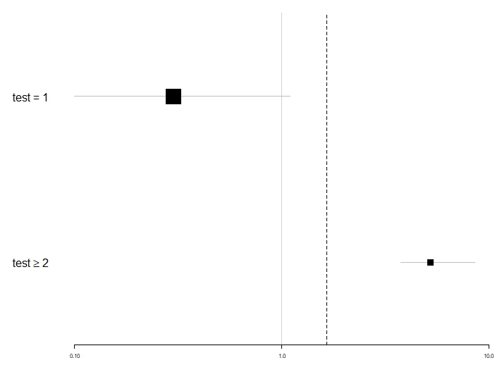
Recently, I've been experiencing difficulties to produce a foresplot and I don't know what could be the reason for this. Could you tell me if this is due to a misuse of your package.

Below are the parameters of my session. I also attach a capture of the resulting graph, the script and the data extract used.

• script*

db <- structure(list(varname = c("Restriction de participation", " Hommes",
" Femmes", "Temps d'activité réduit", " Hommes", " Femmes",
"Faible niveau d'éducation", " Hommes", " Femmes", "Sans emploi",
" Hommes", " Femmes", "Ménage pauvre", " Hommes", " Femmes",
"Confiage dans l'enfance", " Hommes", " Femmes", "Faible soutien social",
" Hommes", " Femmes", " "), coef = c("", "1.13", "0.96",
"", "3.22", "0.85", "", "1.72", "0.99", "", "-0.84", "-0.25",
"", "0.65", "0.54", "", "-0.02", "0.19", "", "0.75", "0.76",
""), ci.low = c("", "0.728", "0.575", "", "2.31", "0.434", "",
"1.296", "0.601", "", "-1.401", "-0.78", "", "0.195", "0.085",
"", "-0.446", "-0.206", "", "0.298", "0.355", ""), ci.high = c("",
"1.535", "1.36", "", "4.432", "1.271", "", "2.164", "1.392",
"", "-0.293", "0.272", "", "1.116", "1.001", "", "0.399", "0.582",
"", "1.213", "1.18", ""), pval = c("", "<0.001", "<0.001", "",
"<0.001", "<0.001", "", "<0.001", "<0.001", "", "0.003", "0.348",
"", "0.006", "0.021", "", "0.913", "0.352", "", "0.001", "<0.001",
""), nlab.ph = c("", "123 (59)", "134 (63)", "", "68 (33)", "93 (44)",
"", "126 (61)", "120 (57)", "", "163 (78)", "171 (81)", "", "63 (30)",
"60 (28)", "", "61 (29)", "85 (40)", "", "67 (32)", "91 (43)",
""), nlab.pt = c("", "67 (32)", "84 (40)", "", "4 (2)", "55 (26)",
"", "45 (22)", "69 (33)", "", "184 (88)", "178 (84)", "", "39 (19)",
"40 (19)", "", "62 (30)", "76 (36)", "", "39 (19)", "55 (26)",
""), status.lab = c("Personnes handicapées (PH) vs Personnes non handicapées (PnH)",
"Personnes handicapées (PH) vs Personnes non handicapées (PnH)",
"Personnes handicapées (PH) vs Personnes non handicapées (PnH)",
"Personnes handicapées (PH) vs Personnes non handicapées (PnH)",
"Personnes handicapées (PH) vs Personnes non handicapées (PnH)",
"Personnes handicapées (PH) vs Personnes non handicapées (PnH)",
"Personnes handicapées (PH) vs Personnes non handicapées (PnH)",
"Personnes handicapées (PH) vs Personnes non handicapées (PnH)",
"Personnes handicapées (PH) vs Personnes non handicapées (PnH)",
"Personnes handicapées (PH) vs Personnes non handicapées (PnH)",
"Personnes handicapées (PH) vs Personnes non handicapées (PnH)",
"Personnes handicapées (PH) vs Personnes non handicapées (PnH)",
"Personnes handicapées (PH) vs Personnes non handicapées (PnH)",
"Personnes handicapées (PH) vs Personnes non handicapées (PnH)",
"Personnes handicapées (PH) vs Personnes non handicapées (PnH)",
"Personnes handicapées (PH) vs Personnes non handicapées (PnH)",
"Personnes handicapées (PH) vs Personnes non handicapées (PnH)",
"Personnes handicapées (PH) vs Personnes non handicapées (PnH)",
"Personnes handicapées (PH) vs Personnes non handicapées (PnH)",
"Personnes handicapées (PH) vs Personnes non handicapées (PnH)",
"Personnes handicapées (PH) vs Personnes non handicapées (PnH)",
"Personnes handicapées (PH) vs Personnes non handicapées (PnH)"
), coef.lab = c("", "1.13[0.728;1.535]", "0.96[0.575;1.36]",
"", "3.22[2.31;4.432]", "0.85[0.434;1.271]", "", "1.72[1.296;2.164]",
"0.99[0.601;1.392]", "", "-0.84[-1.401;-0.293]", "-0.25[-0.78;0.272]",
"", "0.65[0.195;1.116]", "0.54[0.085;1.001]", "", "-0.02[-0.446;0.399]",
"0.19[-0.206;0.582]", "", "0.75[0.298;1.213]", "0.76[0.355;1.18]",
"")), row.names = c(NA, -22L), class = c("tbl_df", "tbl", "data.frame"
))

table.text <- cbind(
c("Caracteristique",db$varname),
c("PH (%)",db$nlab.ph),
c("PnH (%)",db$nlab.pt),
c("Coef",db$coef),
c("p-value",db$pval)
)

forestplot(labeltext=table.text,
title="PH vs PnH",
fn.ci_norm = c(fpDrawNormalCI,#Entete
fpDrawNormalCI,fpDrawCircleCI,fpDrawNormalCI, #Restriction de participation
fpDrawNormalCI,fpDrawCircleCI,fpDrawNormalCI, #Temps d'activité réduit
fpDrawNormalCI,fpDrawNormalCI,fpDrawCircleCI, #Faible niveau d'éducation
fpDrawNormalCI,fpDrawCircleCI,fpDrawNormalCI, #Sans emploi
fpDrawNormalCI,fpDrawCircleCI,fpDrawNormalCI, #Ménage pauvre
fpDrawNormalCI,fpDrawCircleCI,fpDrawNormalCI, #Confiage dans l'enfance
fpDrawNormalCI,fpDrawCircleCI,fpDrawNormalCI, #Faible soutien social
fpDrawNormalCI), #Pieds de page
xlab="Coefficient adjusté sur le groupe d'âge (Coef)",
graph.pos = ncol(table.text),
mean=c(NA,db$coef),
lower=c(NA,db$ci.low),
upper=c(NA,db$ci.high),
is.summary = c(TRUE,rep(FALSE,nrow(table.text)-2),TRUE),
hrzl_lines=list("2"=gpar(lty=1,lwd=2),
"23"=gpar(lty=2,lwd=1,columns=c(1:(ncol(table.text)-1),ncol(table.text)+1))),
zero=0,line.margin = .1,cex=0.9,lwd.ci=2,boxsize = .25,
ci.vertices = TRUE, colgap=unit(3,"mm"),
clip=c(-2,5),xticks = c(-2,-1.5,-1,-0.5,0,0.5,1,1.5,2,2.5,3,3.5,4,4.5,5),
grid=gpar(lty=3,lwd=1,col="gray75"),
txt_gp=fpTxtGp(label = gpar(cex=0.75),ticks=gpar(cex=0.5),xlab = gpar(cex=0.6,fontface="bold")),
summary=list("1"=list(gpar(cex=0.7,fontface="bold"),gpar(cex=0.7,fontface="bold"),
gpar(cex=0.7,fontface="bold"),gpar(cex=0.7,fontface="bold"),
gpar(cex=0.65,fontface="bold")),
"23"=list(gpar(cex=0.5,fontface="italic"),gpar(cex=0.5,fontface="italic"),
gpar(cex=0.5,fontface="italic"),gpar(cex=0.5,fontface="italic"),
gpar(cex=0.5,fontface="italic"))),
col=fpColors(box="black", lines="black", zero = "gray25",summary="black")
)

• Info session

R version 3.5.3 (2019-03-11)
Platform: x86_64-apple-darwin15.6.0 (64-bit)
Running under: macOS 10.15.3

Matrix products: default
BLAS: /System/Library/Frameworks/Accelerate.framework/Versions/A/Frameworks/vecLib.framework/Versions/A/libBLAS.dylib
LAPACK: /Library/Frameworks/R.framework/Versions/3.5/Resources/lib/libRlapack.dylib

locale:
[1] en_US.UTF-8/en_US.UTF-8/en_US.UTF-8/C/en_US.UTF-8/en_US.UTF-8

attached base packages:
[1] grid stats graphics grDevices utils datasets methods base

other attached packages:
[1] forcats_0.4.0 stringr_1.4.0 dplyr_0.8.4 purrr_0.3.3 readr_1.3.1 tidyr_1.0.2
[7] tibble_2.1.3 tidyverse_1.3.0 ggplot2_3.2.1 ggpubr_0.2.4 finalfit_0.9.7 forestplot_1.9
[13] FactoMineR_2.0 checkmate_2.0.0 texreg_1.36.23 magrittr_1.5

loaded via a namespace (and not attached):
[1] httr_1.4.1 jsonlite_1.6.1 splines_3.5.3 modelr_0.1.5 rmeta_3.0
[6] Formula_1.2-3 assertthat_0.2.1 latticeExtra_0.6-28 cellranger_1.1.0 ggrepel_0.8.1
[11] pillar_1.4.3 backports_1.1.5 lattice_0.20-38 glue_1.3.1 digest_0.6.25
[16] RColorBrewer_1.1-2 ggsignif_0.6.0 rvest_0.3.5 minqa_1.2.4 colorspace_1.4-1
[21] htmltools_0.4.0 Matrix_1.2-18 pkgconfig_2.0.3 broom_0.5.4 haven_2.2.0
[26] scales_1.1.0 dummies_1.5.6 lme4_1.1-21 htmlTable_1.13.3 generics_0.0.2
[31] withr_2.1.2 pan_1.6 nnet_7.3-12 lazyeval_0.2.2 cli_2.0.1
[36] readxl_1.3.1 survival_3.1-8 crayon_1.3.4 mitml_0.3-7 mice_3.7.0
[41] fansi_0.4.1 fs_1.3.1 nlme_3.1-143 MASS_7.3-51.4 xml2_1.2.2
[46] foreign_0.8-72 tools_3.5.3 data.table_1.12.8 hms_0.5.3 lifecycle_0.1.0
[51] reprex_0.3.0 munsell_0.5.0 cluster_2.1.0 packrat_0.5.0 flashClust_1.01-2
[56] compiler_3.5.3 rlang_0.4.4 nloptr_1.2.1 rstudioapi_0.11 htmlwidgets_1.5.1
[61] leaps_3.1 base64enc_0.1-3 boot_1.3-23 gtable_0.3.0 DBI_1.0.0
[66] R6_2.4.1 lubridate_1.7.4 gridExtra_2.3 knitr_1.26 Hmisc_4.3-0
[71] jomo_2.6-10 stringi_1.4.6 parallel_3.5.3 Rcpp_1.0.3 vctrs_0.2.3
[76] rpart_4.1-15 acepack_1.4.1 scatterplot3d_0.3-41 dbplyr_1.4.2 tidyselect_1.0.0
[81] xfun_0.11

Hi All,

I am trying to draw a forest plot with below data. It returns error, how can I handle this? Thank you

Error in prFpConvertMultidimArray(mean) : 
  Sorry did not manage to correctly identify the upper/lower boundaries from the input matrix.

mean lower upper
1.10 0.98 1.20
1.10 1.00 1.10
1.10 1.01 1.10

In the forestplot.pdf, I saw this:"If you have several values per row in a forestplot you can set a color to a vector where the first value represents the first line/box, second the second line/box etc."

I wanted to use different colors to display my 4 values, and I set this:

col = fpColors(lines=c('red','blue','black','grey'), box=c('red','blue','black','grey'), zero = "black")

But all the values' color turn to red, rather than the first row in red, the second in blue etc. I don't know why..

Your help is highly appreciated.

The forestplot function print the plot directly to the screen and unable to use ggsave function to save the plot. Also work with plot arranging etc. Might be a good idea to add grid.grab() at the end of drawForestplotObject function to return a gTree object.

Apologies in advance if this should be two separate issues.

Would it be possible to add a method to position the title centrally over wherever the plot is displayed? Here a couple of examples I have produced but, at the moment, the text directly over the plot is hard coded (position-wise) using grid.text:

And also:

Similarly, would it be possible to add a way to label the bottom axis? Here is another forest plot (from a previous issue I have raised) but I am have to hard code the positions of both bits of text (Favour X and Favours Y):

Please let me know if you need anything further from me.

Hello,

Thank you for this amazing package! It's working fine after the latest update, except for one thing I'm unable to fix - the zero line, which previously was working, does not show anymore.

I tried to use the default settings and to play around with settings (e.g. fpColors(zero="black"), zero=1, zero=0). Nothing seems to have an impact.

Do you have any suggestions? Happy to provide further info & a reproducible example if useful.

Hi,

there's one thing I'd like to be able to do with the forestplot() function... there is a little paper giving recommendations on how to set up forest plots:
http://dx.doi.org/10.1186/2046-4053-1-34
They recommend to show the overall mean as a diamond (as usual) and also the prediction interval as a bar (see Fig. 1c). I would like to follow their recommendation, which would mean that (a) I need a function to plot the bar-shaped interval, and (b) I need to be able to specify more than one "fn.ci_sum" argument, e.g. an argument that looks something like:

fn.ci_sum = c(fpDrawDiamondCI, fpDrawBarCI)

I sketched a "fpDrawBarCI()" function (which I essentially mostly copy/pasted from the "fpDrawDiamondCI()" function):

fpDrawBarCI <- function (lower_limit, estimate, upper_limit, size, col, y.offset = 0.5, ...) 
{
  size <- ifelse(is.unit(size), convertUnit(size, unitTo = "npc", valueOnly = TRUE), size) * 0.9
  grid.polygon(x = unit(c(lower_limit, upper_limit, upper_limit, lower_limit), "native"),
               y = unit(y.offset + 0.5*c(1, 1, -1, -1)* size, "npc"),
               gp = gpar(fill = col, col = col))
}

which seems to do the trick; but at the moment I only seem to be able to have both as diamonds or both as bars... Would such a change be possible?

Please would it be possible include an option to draw a border around plot please? Something like the following:

Thanks again!

I have a data frame of mean, lower and upper, first row is NA's and there are 57 rows. Corresponding label text has 57 rows, and first row is col title. When I run the function it gave this error msg below. When subset to the first 35 rows, it runs OK. When removing the NA rows, it runs OK.

Error in if (any(textHeight * (nr + 0.5) * 1.5 < info)) info <- textHeight * :
missing value where TRUE/FALSE needed

Hi,

I wonder if it is possible to add arrows pointing to left and right with corresponding captions below the x-axis like in the following image.

Thanks!

[Source: Stackoverflow]

Sorry to bother you again. :-) I absolutely love this package but when using a list for labeltext (e.g., because of expressions such as a greater equal sign), it is not possible to modify the graph position as flexible when labeltext is a matrix. This is very well described in the help function but is there any way to modify that? What would be the best way to tackle that?

I was already thinking of combining two plots (1 without a graph and a 2nd with graph) using

grid.newpage()
pushViewport(viewport(layout = grid.layout(1, 2,.. etc.

but I get an error message when I do not inlcude mean, lower and upper.

Hello.

I would like to make a forest plot that has each row in a different color. By each row, I mean the boxes and the respective confidence intervals.

Taking an example from the vignette [https://cran.r-project.org/web/packages/forestplot/vignettes/forestplot.html],

library(forestplot)
# Cochrane data from the 'rmeta'-package
cochrane_from_rmeta <- 
  structure(list(
    mean  = c(NA, NA, 0.578, 0.165, 0.246, 0.700, 0.348, 0.139, 1.017, NA, 0.531), 
    lower = c(NA, NA, 0.372, 0.018, 0.072, 0.333, 0.083, 0.016, 0.365, NA, 0.386),
    upper = c(NA, NA, 0.898, 1.517, 0.833, 1.474, 1.455, 1.209, 2.831, NA, 0.731)),
    .Names = c("mean", "lower", "upper"), 
    row.names = c(NA, -11L), 
    class = "data.frame")

tabletext<-cbind(
  c("", "Study", "Auckland", "Block", 
    "Doran", "Gamsu", "Morrison", "Papageorgiou", 
    "Tauesch", NA, "Summary"),
  c("Deaths", "(steroid)", "36", "1", 
    "4", "14", "3", "1", 
    "8", NA, NA),
  c("Deaths", "(placebo)", "60", "5", 
    "11", "20", "7", "7", 
    "10", NA, NA),
  c("", "OR", "0.58", "0.16", 
    "0.25", "0.70", "0.35", "0.14", 
    "1.02", NA, "0.53"))

forestplot(tabletext, 
           cochrane_from_rmeta,new_page = TRUE,
           is.summary=c(TRUE,TRUE,rep(FALSE,8),TRUE),
           clip=c(0.1,2.5), 
           xlog=TRUE, 
           col=fpColors(box="royalblue",line="darkblue", summary="royalblue"))

I want each study to have its own color. Auckland can be blue, Block can be red, Doran can be green, and so on.

Is there any way to do this?

Thank you for fantastic package, could you add option to change color of the plotted row depending on the values in the table. Or use a color vector instead of a single value ? I'm trying to grey-out non significant rows as I plot multiple of these side by side.

Dear all,

Please, I need some help about using the xlog=TRUE option.

It is requested to provide the mean, lower, upper, zero, grid and clip already as exponentials, but I find the package is drawing the grid lines at the exponential of the numbers I am already providing as exponentials. As a consequence, the grid lines are in the wrong place.

  structure(list(
    mean  = c(NA, NA, NA, 0.27, 0.47, 0.33, 0.69, 0.86, 0.37, 0.08, 0.44, 0.54, 0.41, NA), 
    lower = c(NA, NA, NA, 0.13, 0.12, 0.19, 0.12, 0.54, 0.17, 0.03, 0.16, 0.06, 0.29, NA),
    upper = c(NA, NA, NA, 0.58, 1.81, 0.60, 3.97, 1.36, 0.81, 0.21, 1.25, 4.50, 0.58, NA)),
    .Names = c("mean", "lower", "upper"), 
    row.names = c(NA, -27L), 
    class = "data.frame")

tabletext<-cbind(
  c("", "AB class", "", "     Aminoglycosides", "     B-lactams", "     Cephalosporins", "     Fenicoles", "     Fluoroquinolones", "     Multiresistance", "     Sulphamides", "     Tetracyclines", "     Tri/Sulpha", "     Subtotal", ""),  
  c("", "OR", "", "0.27", "0.47", "0.33", "0.69", "0.86", "0.37", "0.08", "0.44", "0.54", "0.41", ""),
  c("", "n", "", "4", "3", "2", "3", "4", "2", "3", "4", "3", "5", ""))

xticks <- c(0.1, 0.25, 0.5, 1, 1.5, 2, 3)

forestplot(tabletext,
           graph.pos = 3,
           txt_gp = fpTxtGp(label = gpar(fontsize=10)),
           hrzl_lines = list("3" = gpar(lty=1)),
           zero = 1,
           line.margin = .05,
           mean = cbind(metaan[,"mean"]),
           lower = cbind(metaan[,"lower"]),
           upper = cbind(metaan[,"upper"]),
           is.summary=c(FALSE, TRUE, rep(FALSE, 9)),
           col=fpColors(box=c("blue"), summary=c("blue")),
           grid = structure(0.41, 
                            gp = gpar(lty = 2, col = "#CCCCFF")),
           clip=c(0.1, 3),
           xlog=T,
           xticks=xticks,
           xlab="Odds ratio")

When provided the log to get the grid lines at the correct place (e.g. -0.38, or log(0.41)), I get the error message that I should provide all parameters already as exponential.

forestplot(tabletext,
           graph.pos = 3,
           txt_gp = fpTxtGp(label = gpar(fontsize=10)),
           hrzl_lines = list("3" = gpar(lty=1)),
           zero = 1,
           line.margin = .05,
           mean = cbind(metaan[,"mean"]),
           lower = cbind(metaan[,"lower"]),
           upper = cbind(metaan[,"upper"]),
           is.summary=c(FALSE, TRUE, rep(FALSE, 9)),
           col=fpColors(box=c("blue"), summary=c("blue")),
           grid = structure(-0.39, 
                            gp = gpar(lty = 2, col = "#CCCCFF")),
           clip=c(0.1, 3),
           xlog=T,
           xticks=xticks,
           xlab="Odds ratio")

Error in forestplot.default(tabletext, graph.pos = 3, txt_gp = fpTxtGp(label = gpar(fontsize = 10)),  : 
  All argument values (mean, lower, upper, zero, grid and clip) should be provided as exponentials when using the log scale. This is an intentional break with the original forestplot function in order to simplify other arguments such as ticks, clips, and more.

I have tried including the grid numbers as lists, but I always encounter the same error message either if I provide the numbers as exponentials (grid misplaced) or as log (error message).

I am wondering what I am doing wrong and if there is any other way to get the grid lines in the correct place.

Thanks in advance,

Magda.

Issue 1: Unable to apply different parameters to elements using a list of parameter within

"fpTxtGp(label = gpar( cex = List of values for individual elements goes here) )

Can you please specify any instructions in the package's pdf file?

Issue 2: Error using "font" of "fontface" within gpar in fpTxtGp. Get the error "Error in validGP(list(...)) :
must specify only one of 'font' and 'fontface' "
The error message is saying that I tried inputting both "font" and "fontface" into gpar, however I only used one of either "font" or "fontface", and get the error message using either one.

Hi, thank you for sharing your code. It is really helpful for drawing the forest plot. I am just wondering the argument "boxsize" embedded in the function "forestplot", the default value of the boxsize to present the precision of effect size. Could this boxsize be set to present the weighed (the sample size for corespondent study)?

Hi all,

I am wondering how to create two forest plots within one forestplot object. One possible way would be to connect two forestplot objects once they were saved as png or jpeg. Is there any other better solution?

Thanks.

Kai

Hi there,

Am very new to R, so please forgive my ignorance.

Have managed to set up a forest plot with two sets of confidence bands, and am hoping to be able to add horizontal bands as shown here. But regardless of what "row" I choose, the bands always end up in between my row labels.

An example is shown below:

Regardless of how I tweak the parameters, the bands don't seem to end up in the right place.

hrzl_lines=list("2" = gpar(lwd=40, lineend="butt", col="#99999922"), "4" = gpar(lwd=40, lineend="butt", col="#99999922"), "5" = gpar(lwd=40, lineend="butt", col="#99999922"))

Any help would be much appreciated! Thanks.

Hi, I keep getting the following message when I try to run the script. When I run it with data with 7 rows it ran fine. I am trying to run it with a dataset with 38 rows now.

Thank you!

Error in if (any(textHeight * (nr + 0.5) * 1.5 < info)) info <- textHeight * :
missing value where TRUE/FALSE needed

Example from vignette:

library(forestplot)
Loading required package: grid
Loading required package: magrittr
Loading required package: checkmate
ask <- par(ask = TRUE)

An example of how fpShapesGp works

styles <- fpShapesGp(

• default = gpar(col = "pink", lwd = 2, lineend = "square", linejoin = "mitre"),
  

• grid = list(
  

•     gpar(col = "blue"),
  

•     gpar(col = "black"),
  

•     gpar(col = "blue")
  

• ),
  

• box = list(
  

•     gpar(fill = "black"),
  

•     gpar(fill = "blue"),
  

•     gpar(fill = "black"),
  

•     gpar(fill = "blue")
  

• ),
  

• lines = gpar(lty = "dashed"),
  

• vertices = gpar(lwd = 5, col = "red")
  

• )
  Error in fpShapesGp(default = gpar(col = "pink", lwd = 2, lineend = "square", :
  could not find function "fpShapesGp"

R version 3.6.3 (2020-02-29)
forestplot_1.9

Me and a colleague are observing a strange behaviour when plotting 5 Groups with 5 'Treatments', whereby there are different marker symbols for each 'treatment'. I've modified the example in vignette to demonstrate this.

In this following diagram showing 6 Groups with 5 Treatments (6x5), the markers seem to be placed properly. Markers are grouped by treatments. This is the same behaviour when I tried a 4x4 plot.

However, in the following diagram showing 5 Groups with 5 Treatments (5x5), the markers seem to be categorised by Groups, as opposed to treatments.

Is this the correct behaviour? Thanks.

Hi, I am trying to use the forestplot function for data from a network meta, analysis. When I create the plot it seems to have squashed the x-axis and confidence intervals as such.

it seems to only have happened after I added my P-Value column as without it it appears like this

I have tried playing around viewport settings to no avail

Here is the code I have for the plot including P-Values

net5_forestplot <- forestplot(mean = as.numeric(graphtable5[,4]),
                              upper = as.numeric(graphtable5[,6]),
                              lower = as.numeric(graphtable5[,5]),
                              labeltext = graphtable5[,1:3],
                              is.summary = c(T,T,rep(F,3),T,rep(F,3),T,rep(F,3),T,rep(F,3)),
                              hrzl_lines = list("2" = gpar(lwd=1, columns=1:3, col = "#000044"), 
                                                "3" = gpar(lwd=1, columns=1:3, col = "#000044"),
                                                "6" = gpar(lwd=1, columns=1:3, col = "#000044"),
                                                "7" = gpar(lwd=1, columns=1:3, col = "#000044"),
                                                "10" = gpar(lwd=1, columns=1:3, col = "#000044"),
                                                "11" = gpar(lwd=1, columns=1:3, col = "#000044"),
                                                "14" = gpar(lwd=1, columns=1:3, col = "#000044"),
                                                "15" = gpar(lwd=1, columns=1:3, col = "#000044")),
                              txt_gp=fpTxtGp(label=gpar(cex=1.1),
                                             ticks=gpar(cex=1.1),
                                             xlab=gpar(cex = 1.2),
                                             title=gpar(cex = 1.2)),
                            col=fpColors(box="royalblue", lines="darkblue", hrz_lines = "#444444", zero = "gray50"),
                              cex=0.9, lineheight = "auto", boxsize=0.5, colgap=unit(6,"mm"),
                              lwd.ci=2, ci.vertices=TRUE, ci.vertices.height = 0.4,
                              xlab = "<-- Favours Comparator   Favours Treatment --->",
                              title = expression(paste("Procedure Duration, 14 Trials, ", italic("I"^"2"), "= 91%")))

I am wondering if you may be able to help me? I'm sorry if it's a stupid question and there is an easy solution.

I have another suggestion; I think it would be useful to be able to suppress the vertical line (which is set through the zero argument) by (e.g.) specifying zero=FALSE or/and zero=NA.

Not a bug, thank you

(content removed because relevant to upcoming publication)