bayesAB provides a suite of functions that allow the user to analyze A/B test data in a Bayesian framework. bayesAB is intended to be a drop-in replacement for common frequentist hypothesis test such as the t-test and chi-sq test.
Bayesian methods provide several benefits over frequentist methods in the context of A/B tests - namely in interpretability. Instead of p-values you get direct probabilities on whether A is better than B (and by how much). Instead of point estimates your posterior distributions are parametrized random variables which can be summarized any number of ways.
While Bayesian AB tests are still not immune to peeking in the broadest sense, you can use the 'Posterior Expected Loss' provided in the package to draw conclusions at any point with respect to your threshold for error.
The general bayesAB workflow is as follows:
- Decide how you want to parametrize your data (Poisson for counts of email submissions, Bernoulli for CTR on an ad, etc.)
- Use our helper functions to decide on priors for your data (
?bayesTest,?plotDistributions) - Fit a
bayesTestobject- Optional: Use
combineto munge together severalbayesTestobjects together for an arbitrary / non-analytical target distribution
- Optional: Use
print,plot, andsummaryto interpret your results- Determine whether to stop your test early given the Posterior Expected Loss in
summaryoutput
- Determine whether to stop your test early given the Posterior Expected Loss in
Optionally, use banditize and/or deployBandit to turn a pre-calculated (or empty) bayesTest into a multi-armed bandit that can serve recipe recommendations and adapt as new data comes in.
Note, while bayesAB was designed to exploit data related to A/B/etc tests, you can use the package to conduct Bayesian analysis on virtually any vector of data, as long as it can be parametrized by the available functions.
Get the latest stable release from CRAN:
install.packages("bayesAB")Or the dev version straight from Github:
install.packages("devtools")
devtools::install_github("frankportman/bayesAB", build_vignettes = TRUE)Some useful links from my blog with bayesAB examples (and pictures!!):
For a more in-depth look please check the package vignettes with browseVignettes(package = "bayesAB") or the pre-knit HTML version on CRAN here. Brief example below. Run the following code for a quick overview of bayesAB:
library(bayesAB)
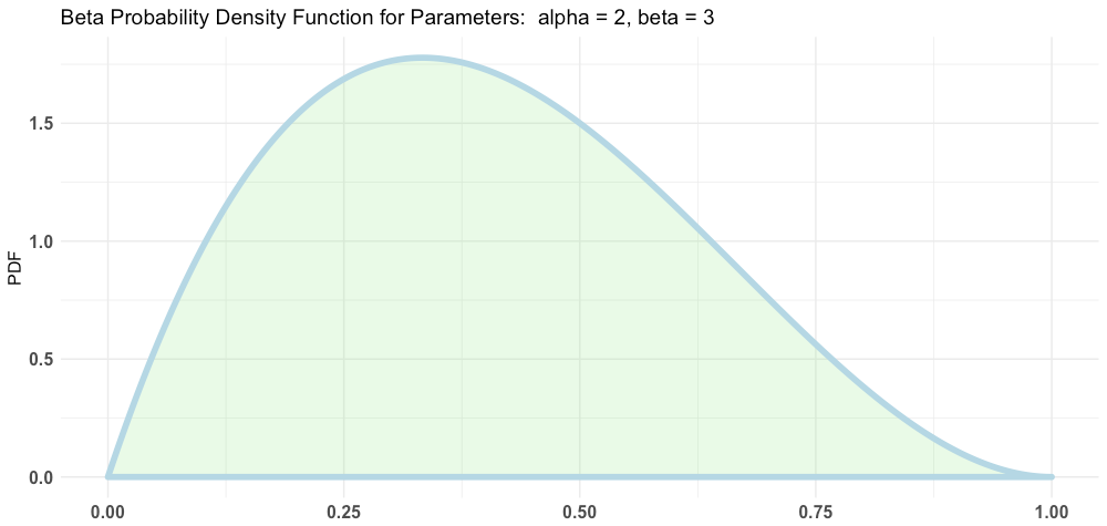
# Choose bernoulli test priors
plotBeta(2, 3)
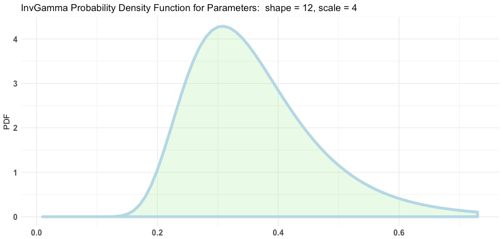
# Choose normal test priors
plotInvGamma(12, 4)
A_binom <- rbinom(100, 1, .5)
B_binom <- rbinom(100, 1, .55)
# Fit bernoulli test
AB1 <- bayesTest(A_binom,
B_binom,
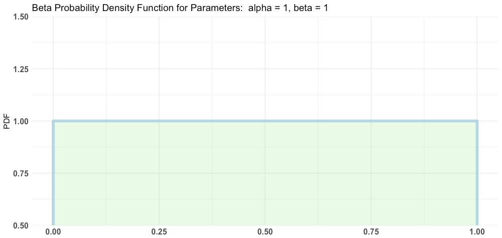
priors = c('alpha' = 1, 'beta' = 1),
distribution = 'bernoulli')
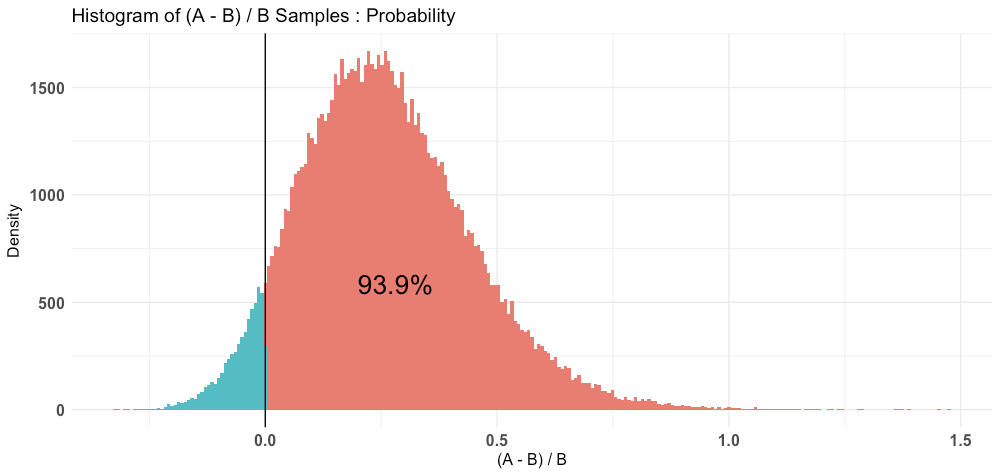
plot(AB1)

print(AB1)
--------------------------------------------
Distribution used: bernoulli
--------------------------------------------
Using data with the following properties:
           A    B
Min.    0.00 0.00
1st Qu. 0.00 0.00
Median  1.00 0.00
Mean    0.55 0.44
3rd Qu. 1.00 1.00
Max.    1.00 1.00
--------------------------------------------
Priors used for the calculation:
$alpha
[1] 1

$beta
[1] 1

--------------------------------------------
Calculated posteriors for the following parameters:
Probability
--------------------------------------------
Monte Carlo samples generated per posterior:
[1] 1e+05
summary(AB1)
Quantiles of posteriors for A and B:

$Probability
$Probability$A
       0%       25%       50%       75%      100%
0.3330638 0.5159872 0.5496165 0.5824940 0.7507997

$Probability$B
       0%       25%       50%       75%      100%
0.2138149 0.4079403 0.4407221 0.4742673 0.6369742


--------------------------------------------

P(A > B) by (0)%:

$Probability
[1] 0.93912

--------------------------------------------

Credible Interval on (A - B) / B for interval length(s) (0.9) :

$Probability
         5%         95%
-0.01379425  0.58463290

--------------------------------------------

Posterior Expected Loss for choosing A over B:

$Probability
[1] 0.03105786