Helper functions to automate Exploratory Data Analysis. The focus is mainly on typical Machine Learning datasets, where there is a target variable (numerical or categorical) and the aim of EDA is to get a sense of the data and whether the variables may be useful for the prediction or not.

In order to perform automatic EDA on your dataset, you need to import the library, define wich variables are numerical and which are categorical, and which one is the target. In order for the calculation of the association metrics to work properly, it is also suggested that all missing values for the categorical variables be replaced by one or more explicit values. The method summaryEDA will compute summaries and charts and output a dictionary of all the data generated.

from MLAutoEDA import MLAutoEDA

numerical_vars = ['Age', 'SibSp', 'Fare']
categorical_vars = ['Pclass', 'Sex', 'Ticket', 'Cabin', 'Embarked']
target = 'Survived'

dataframe[categorical_vars] = dataframe[categorical_vars].astype("category")
for c in categorical_vars:
    if ("Unknown" not in dataframe[c].cat.categories):
        dataframe.loc[:, c] = dataframe[c].cat.add_categories("Unknown").fillna("Unknown")

auto_eda = MLAutoEDA(dataframe, numerical_vars, categorical_vars, target, target_type)
summary_dict = auto_eda.summaryEDA()

The dictionary will contain the summary data for various combination of the variables and the target, as well as the matplotlib figure and axes handles so that they can be rendered and modified afterwards. You can also save the dictionary as a pickle file to avoid computing it multiple times.

This library produces different types of charts and summaries depending on the combination of the types of variables to plot. The library handles univariate, bi-variate (variable vs target) and tri-variate (2 variables vs target) plots.

The summary dictionary contains the summary of associations between variables, as well as the figure and axis handles for the association matrix:

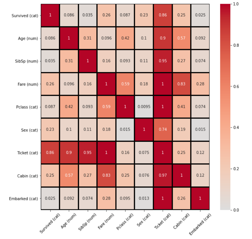
The association matrix handles both numerical and categorical variables:

• For numerical vs numerical variables, the absolute value of the Pearson's correlation coefficient is computed. The absolute value ensures the range is between 0 and 1 like the other quantities.
• For numerical vs categorical variables, the correlation ratio is computed.
• For categorical vs categorical variables, the Theil's U coefficient is computed. Be aware that this is not a symmetrical measure.

It is possible to acces the matrix directly from the summary dictionary:

summary_dict['associations']['df_corr']
summary_dict['associations']['df_corr_ordered']

df_corr_ordered is the unstacked version of the df_corr matrix, ordered from higher to lower value.

The univariate graphs for numerical variables are a histogram of the values, along with a kde distribution, and a boxplot:

The summary data for this case is the standard summary provided by pandas.

The univariate graph for categorical variables is a countplot:

The summary is a value_counts normalized and unnormalized.

In this case, a scatterplot is produced.

The summary is a combination of the single-variable summaries.

For a numerical variable vs. a categorical target, the library produces a grouped boxplot and a kde plot for each category of the target. The boxplot also features the overall mean and median of the variable, for comparison.

The summary is an overall describe for the numerical variable, along with a describe for each value of the target variable.

This produces two plots: a boxplot for the distribution of the target for each value of the categorical variable, and a kde plot showing the distributions. The boxplot also features the overall mean and median of the target, for comparison

The summary is an overall describe for the target, along with a describe for each value of the categorical variable.

This produces two plots: a bar plot, grouped by the target, with the percentages of records in each group, and a countplot grouped by the target variable. In the percentage plot, the overall proportions for each level of the target variable are marked with vertical dashed lines, for comparison. For instance, in the following graph it is very easy to see that the survival rate for first class passengers is much higher than the base rate, whereas it is quite lower for 3rd class.

The summary consists of two crosstabs, one with a count and another one with percentages computed over the target.

This produces a hexbin plot where the value of the target variable is represented as a color gradient.

The summary is a describe statement for each of the variables.

This produces a scatterplot of the two numerical variables, with a hue for each level of the target.

The summary is a describe statement for each of the numerical variables, along with describe statements for each value of the target.

This produces a grouped boxplot for the distribution of the target variable.

The summary is a describe statement for each combination of the two categorical variables.

This produces two graphs for each value of the target variable. On the left, a heatmap with the proportion of records with that target value for each combination of the two categorical variables. On the left, the same heatmap, with the values "shifted" with respect to the overall rate of the target variable. For instance, in the first line of the following two graphs, one can see that the percentage of men travelling first class that would not survive is 63%, which represents a 1.5% increase with respect to the overall death rate. Note of caution: since the percentages are calculated over the target, given one heatmap those do not sum to 1. For the percentages to sum to 1, one needs to look only at the left side graphs, and sum up the corresponding squares of both graphs. For instance, for men in first class the death rate is 0.63 and the survival rate is 0.37, which sums to 1

The summaries are two hierarchical crosstabs, where the target is in the columns. The first one is for the counts and the second one is for percentages.

This produces a scatterplot of the numerical variables vs the target, where the hue correspond to the categorical one.

The summary is a describe statement for the two numerical variables, for each possible value of the categorical one.

This produces a boxplot like the following one, with the overall mean and median of the numerical variable to provide reference.

The summary is a describe statement for the numerical variable, for each possible combination of the two categorical ones.