Sometimes you may wish to find the mean, median, min, or max of a column feature. For example, there could be a customer relational database that you've been working with and you may wonder if there are differences in overall sales across offices or regions. We can use aggregate functions in SQL to assist with performing these analyses.
You will be able to:
- Describe the relationship between aggregate functions and
GROUP BYstatements - Use
GROUP BYstatements in SQL to apply aggregate functions like:COUNT,MAX,MIN, andSUM - Create an alias in a SQL query
- Use the
HAVINGclause to compare different aggregates - Compare the difference between the
WHEREandHAVINGclause
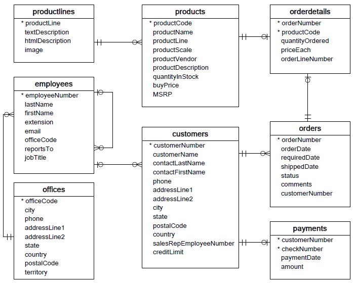
Once again we will be using this database, with 8 tables relating to customers, orders, employees, etc.
As usual, start by creating a connection to the database. We will also import pandas in order to display the results in a convenient format.
import sqlite3
import pandas as pd
conn = sqlite3.Connection('data.sqlite')Let's start by looking at some GROUP BY statements to aggregate our data. The GROUP BY clause groups records into summary rows and returns one record for each group.
Typically, GROUP BY also involves an aggregate function (COUNT, AVG, etc.).
Lastly, GROUP BY can group by one column or multiple columns.
One of the most common uses of GROUP BY is to count the number of records in each group. To do that, we'll also use the COUNT aggregate function.
q = """
SELECT country, COUNT(*)
FROM customers
GROUP BY country
;
"""
# Displaying just the first 10 countries for readability
pd.read_sql(q, conn).head(10).dataframe tbody tr th {
vertical-align: top;
}
.dataframe thead th {
text-align: right;
}
| country | COUNT(*) | |
|---|---|---|
| 0 | Australia | 5 |
| 1 | Austria | 2 |
| 2 | Belgium | 2 |
| 3 | Canada | 3 |
| 4 | Denmark | 2 |
| 5 | Finland | 3 |
| 6 | France | 12 |
| 7 | Germany | 13 |
| 8 | Hong Kong | 1 |
| 9 | Ireland | 2 |
Cool, we have the number of customers per country!
Why did we pass in * to COUNT(*)?
COUNT is a function that is being invoked, similar to a function in Python. When we say to count *, we mean count every row containing non-null column values.
You will also see examples using COUNT(1), which counts every row regardless of whether it contains non-null column values, or something like COUNT(customerNumber), which just counts whether some particular column is non-null.
Most of the time this does not make a significant difference in the results produced or the processing speed, since databases have optimizers designed for this purpose. But it is useful to be able to recognize the various forms.
Another thing to be aware of is that instead of specifying an actual column name to group by, we can group the data using the index of one of the columns already specified in the SELECT statement. These are 1-indexed (unlike Python, which is 0-indexed). So an alternative way to write the previous query would be:
q = """
SELECT country, COUNT(*)
FROM customers
GROUP BY 1
;
"""
# Displaying just the first 10 countries for readability
pd.read_sql(q, conn).head(10).dataframe tbody tr th {
vertical-align: top;
}
.dataframe thead th {
text-align: right;
}
| country | COUNT(*) | |
|---|---|---|
| 0 | Australia | 5 |
| 1 | Austria | 2 |
| 2 | Belgium | 2 |
| 3 | Canada | 3 |
| 4 | Denmark | 2 |
| 5 | Finland | 3 |
| 6 | France | 12 |
| 7 | Germany | 13 |
| 8 | Hong Kong | 1 |
| 9 | Ireland | 2 |
An alias is a shorthand for a table or column name. Aliases reduce the amount of typing required to enter a query, and can result in both queries and results that are easier to read.
Aliases are especially useful with JOIN, GROUP BY, and aggregates (SUM, COUNT, etc.). For example, we could rewrite the previous query like this, so that the count of customers is called customer_count instead of COUNT(*):
q = """
SELECT country, COUNT(*) AS customer_count
FROM customers
GROUP BY country
;
"""
# Displaying just the first 10 countries for readability
pd.read_sql(q, conn).head(10).dataframe tbody tr th {
vertical-align: top;
}
.dataframe thead th {
text-align: right;
}
| country | customer_count | |
|---|---|---|
| 0 | Australia | 5 |
| 1 | Austria | 2 |
| 2 | Belgium | 2 |
| 3 | Canada | 3 |
| 4 | Denmark | 2 |
| 5 | Finland | 3 |
| 6 | France | 12 |
| 7 | Germany | 13 |
| 8 | Hong Kong | 1 |
| 9 | Ireland | 2 |
Other notes on aliases:
- An alias only exists for the duration of the query.
- The keyword
ASis optional in SQLite. So, you could just sayCOUNT(*) customer_countwith the same outcome. Historically some forms of SQL requiredASand others would not work withAS, but most work either way now. In a professional setting you will likely have a style guide indicating whether or not to use it.
Aside from COUNT() some other useful aggregations include:
MIN()MAX()SUM()AVG()
These are mainly useful when working with numeric data.
In the cell below, we calculate various summary statistics about payments, grouped by customer.
q = """
SELECT
    customerNumber,
    COUNT(*) AS number_payments,
    MIN(amount) AS min_purchase,
    MAX(amount) AS max_purchase,
    AVG(amount) AS avg_purchase,
    SUM(amount) AS total_spent
FROM payments
GROUP BY customerNumber
;
"""
pd.read_sql(q, conn).dataframe tbody tr th {
vertical-align: top;
}
.dataframe thead th {
text-align: right;
}
| customerNumber | number_payments | min_purchase | max_purchase | avg_purchase | total_spent | |
|---|---|---|---|---|---|---|
| 0 | 103 | 3 | 1676.14 | 14571.44 | 7438.120000 | 22314.36 |
| 1 | 112 | 3 | 14191.12 | 33347.88 | 26726.993333 | 80180.98 |
| 2 | 114 | 4 | 7565.08 | 82261.22 | 45146.267500 | 180585.07 |
| 3 | 119 | 3 | 19501.82 | 49523.67 | 38983.226667 | 116949.68 |
| 4 | 121 | 4 | 1491.38 | 50218.95 | 26056.197500 | 104224.79 |
| ... | ... | ... | ... | ... | ... | ... |
| 93 | 486 | 3 | 5899.38 | 45994.07 | 25908.863333 | 77726.59 |
| 94 | 487 | 2 | 12573.28 | 29997.09 | 21285.185000 | 42570.37 |
| 95 | 489 | 2 | 7310.42 | 22275.73 | 14793.075000 | 29586.15 |
| 96 | 495 | 2 | 6276.60 | 59265.14 | 32770.870000 | 65541.74 |
| 97 | 496 | 3 | 30253.75 | 52166.00 | 38165.730000 | 114497.19 |
98 rows × 6 columns
Similar to before we used GROUP BY and aggregations, we can use WHERE to filter the data. For example, if we only wanted to include payments made in 2004:
q = """
SELECT
    customerNumber,
    COUNT(*) AS number_payments,
    MIN(amount) AS min_purchase,
    MAX(amount) AS max_purchase,
    AVG(amount) AS avg_purchase,
    SUM(amount) AS total_spent
FROM payments
WHERE strftime('%Y', paymentDate) = '2004'
GROUP BY customerNumber
;
"""
pd.read_sql(q, conn).dataframe tbody tr th {
vertical-align: top;
}
.dataframe thead th {
text-align: right;
}
| customerNumber | number_payments | min_purchase | max_purchase | avg_purchase | total_spent | |
|---|---|---|---|---|---|---|
| 0 | 103 | 2 | 1676.14 | 6066.78 | 3871.460 | 7742.92 |
| 1 | 112 | 2 | 14191.12 | 33347.88 | 23769.500 | 47539.00 |
| 2 | 114 | 2 | 44894.74 | 82261.22 | 63577.980 | 127155.96 |
| 3 | 119 | 2 | 19501.82 | 47924.19 | 33713.005 | 67426.01 |
| 4 | 121 | 2 | 17876.32 | 34638.14 | 26257.230 | 52514.46 |
| ... | ... | ... | ... | ... | ... | ... |
| 83 | 486 | 2 | 5899.38 | 45994.07 | 25946.725 | 51893.45 |
| 84 | 487 | 1 | 12573.28 | 12573.28 | 12573.280 | 12573.28 |
| 85 | 489 | 1 | 7310.42 | 7310.42 | 7310.420 | 7310.42 |
| 86 | 495 | 1 | 6276.60 | 6276.60 | 6276.600 | 6276.60 |
| 87 | 496 | 1 | 52166.00 | 52166.00 | 52166.000 | 52166.00 |
88 rows × 6 columns
Some additional notes:
- Look at the difference in the first row values. It appears that customer 103 made 3 payments in the database overall, but only made 2 payments in 2004. So this row still represents the same customer as in the previous query, but it contains different aggregated information about that customer.
- This returned 88 rows rather than 98, because some of the customers are present in the overall database but did not make any purchases in 2004.
- Recall that you can filter based on something in a
WHEREclause even if you do notSELECTthat column. We are not displaying thepaymentDatevalues because this would not make much sense in aggregate, but we can still use that column for filtering.
Finally, we can also filter our aggregated views with the HAVING clause. The HAVING clause works similarly to the WHERE clause, except it is used to filter data selections on conditions after the GROUP BY clause.
For example, if we wanted to filter to only select aggregated payment information about customers with average payment amounts over 50,000:
q = """
SELECT
    customerNumber,
    COUNT(*) AS number_payments,
    MIN(amount) AS min_purchase,
    MAX(amount) AS max_purchase,
    AVG(amount) AS avg_purchase,
    SUM(amount) AS total_spent
FROM payments
GROUP BY customerNumber
HAVING avg_purchase > 50000
;
"""
pd.read_sql(q, conn).dataframe tbody tr th {
vertical-align: top;
}
.dataframe thead th {
text-align: right;
}
| customerNumber | number_payments | min_purchase | max_purchase | avg_purchase | total_spent | |
|---|---|---|---|---|---|---|
| 0 | 124 | 9 | 11044.30 | 111654.40 | 64909.804444 | 584188.24 |
| 1 | 141 | 13 | 20009.53 | 120166.58 | 55056.844615 | 715738.98 |
| 2 | 239 | 1 | 80375.24 | 80375.24 | 80375.240000 | 80375.24 |
| 3 | 298 | 2 | 47375.92 | 61402.00 | 54388.960000 | 108777.92 |
| 4 | 321 | 2 | 46781.66 | 85559.12 | 66170.390000 | 132340.78 |
| 5 | 450 | 1 | 59551.38 | 59551.38 | 59551.380000 | 59551.38 |
Note that in most flavors of SQL we can't use an alias in the HAVING clause. This is due to the internal order of execution of the SQL commands. So in most cases outside of SQLite you would need to write that query like this, repeating the aggregation code in the HAVING clause:
q = """
SELECT
    customerNumber,
    COUNT(*) AS number_payments,
    MIN(amount) AS min_purchase,
    MAX(amount) AS max_purchase,
    AVG(amount) AS avg_purchase,
    SUM(amount) AS total_spent
FROM payments
GROUP BY customerNumber
HAVING AVG(amount) > 50000
;
"""
pd.read_sql(q, conn).dataframe tbody tr th {
vertical-align: top;
}
.dataframe thead th {
text-align: right;
}
| customerNumber | number_payments | min_purchase | max_purchase | avg_purchase | total_spent | |
|---|---|---|---|---|---|---|
| 0 | 124 | 9 | 11044.30 | 111654.40 | 64909.804444 | 584188.24 |
| 1 | 141 | 13 | 20009.53 | 120166.58 | 55056.844615 | 715738.98 |
| 2 | 239 | 1 | 80375.24 | 80375.24 | 80375.240000 | 80375.24 |
| 3 | 298 | 2 | 47375.92 | 61402.00 | 54388.960000 | 108777.92 |
| 4 | 321 | 2 | 46781.66 | 85559.12 | 66170.390000 | 132340.78 |
| 5 | 450 | 1 | 59551.38 | 59551.38 | 59551.380000 | 59551.38 |
We can also use the WHERE and HAVING clauses in conjunction with each other for more complex rules.
For example, let's say we want to filter based on customers who have made at least 2 purchases of over 50000 each.
To convert that into SQL logic, that means we first want to limit the records to purchases over 50000 (using WHERE), then after aggregating, limit to customers who have made at least 2 purchases fitting that previous requirement (using HAVING).
q = """
SELECT
    customerNumber,
    COUNT(*) AS number_payments,
    MIN(amount) AS min_purchase,
    MAX(amount) AS max_purchase,
    AVG(amount) AS avg_purchase,
    SUM(amount) AS total_spent
FROM payments
WHERE amount > 50000
GROUP BY customerNumber
HAVING number_payments >= 2
;
"""
pd.read_sql(q, conn).dataframe tbody tr th {
vertical-align: top;
}
.dataframe thead th {
text-align: right;
}
| customerNumber | number_payments | min_purchase | max_purchase | avg_purchase | total_spent | |
|---|---|---|---|---|---|---|
| 0 | 124 | 5 | 55639.66 | 111654.40 | 87509.512 | 437547.56 |
| 1 | 141 | 5 | 59830.55 | 120166.58 | 85024.068 | 425120.34 |
| 2 | 151 | 2 | 58793.53 | 58841.35 | 58817.440 | 117634.88 |
| 3 | 363 | 2 | 50799.69 | 55425.77 | 53112.730 | 106225.46 |
We can also use the ORDER BY and LIMIT clauses in queries containing these complex rules. Say we want to find the customer with the lowest total amount spent, who nevertheless fits the criteria described above. That would be:
q = """
SELECT
    customerNumber,
    COUNT(*) AS number_payments,
    MIN(amount) AS min_purchase,
    MAX(amount) AS max_purchase,
    AVG(amount) AS avg_purchase,
    SUM(amount) AS total_spent
FROM payments
WHERE amount > 50000
GROUP BY customerNumber
HAVING number_payments >= 2
ORDER BY total_spent
LIMIT 1
;
"""
pd.read_sql(q, conn).dataframe tbody tr th {
vertical-align: top;
}
.dataframe thead th {
text-align: right;
}
| customerNumber | number_payments | min_purchase | max_purchase | avg_purchase | total_spent | |
|---|---|---|---|---|---|---|
| 0 | 363 | 2 | 50799.69 | 55425.77 | 53112.73 | 106225.46 |
In this lesson, you learned how to use aggregate functions, aliases, and the HAVING clause to filter selections.


