Creativity is something we closely associate with what it means to be human. But with digital technology now enabling machines to recognize, learn from and respond to humans and the world, an inevitable question follows:

Can machine be creative? And will artificial intelligence ever be able to make art?

Recent art experiments are the use of "generative adversarial networks" (GANs). GANs are "neural networks" that teach themselves through their own experimentation, rather than being programmed by humans. It could be argued that the ability of machines to learn what things look like, and then make convincing new examples, marks the advent of "creative" AI.

I will cover four different methods by which you can create novel arts, solely by code - Neural Style Transfer, Deep Dream, CycleGAN, and Pix2pix.

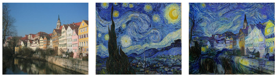
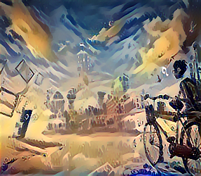
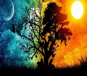
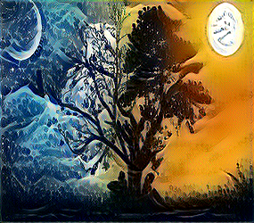
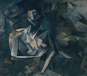
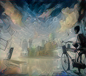
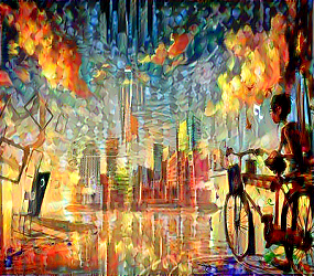
Neural Style Transfer (NST) is one of the most fun techniques in deep learning. As seen below, it merges two images, namely, a "content" image (C) and a "style" image (S), to create a "generated" image (G). The generated image G combines the "content" of the image C with the "style" of image S.

Neural Style Transfer (NST) uses a previously trained convolutional network and builds on top of that. I will be using VGG-19 which has already been trained on the very large ImageNet database. It learned to recognize a variety of low-level features (at the earlier layers) and high-level features (at the deeper layers). Building the NST algorithm takes three steps:

• Content Cost : Jcontent (C, G)
• Style Cost : Jstyle (S, G)
• Total Variation (TV) Cost : Jtv (G)

Putting all together : Jtot (G) = (alpha) * Jcontent (C, G) + (beta) * Jstyle (S, G) + (gamma)* Jtv (G)

Let's delve deeper to know more profoundly what's going on under the hood of these algorithms.

The earlier layers of a ConvNet tend to detect lower-level features such as edges and simple textures, and the later layers tend to detect higher-level features such as more complex textures as well as object classes. Content loss tries to make sure that "generated" image G has similar content as the input image C. For that, we need to choose some layer's activation to represent the content of an image. Practically, we'll get the most visually pleasing results if we choose a layer in the middle of the network - neither too shallow nor too deep. Suppose we picked activations of Conv_3_2 layer to represent the content cost. Now, set the image C as the input to the pre-trained VGG network, and run forward propagation.

Let a(C) be the hidden layer activations which will be a nH * nW * nC tensor. Repeat the same process for the generated image and let a(G) be the corresponding hidden layer activations. Finally, the Content Cost function is defined as follows:

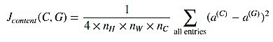
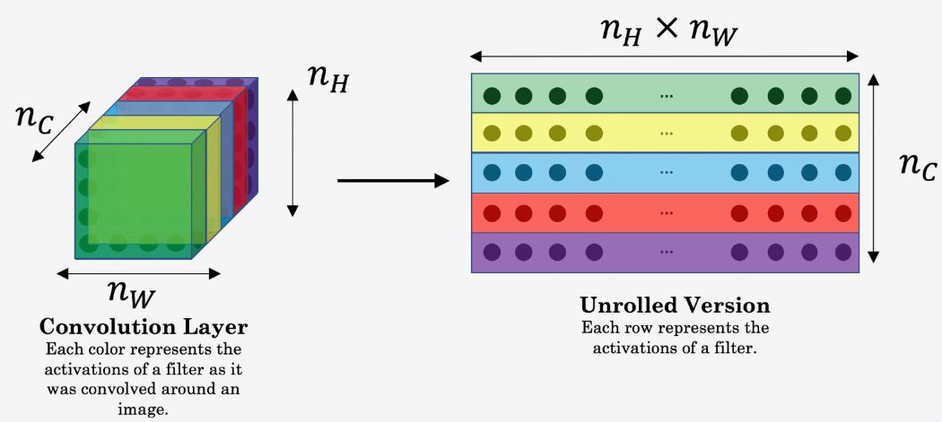
nH, nW, and nC are the height, width, and the number of channels of the hidden layer chosen. In order to compute the cost **J***content* (C, G), it might also be convenient to unroll these 3D volumes into a 2D matrix, as shown below.

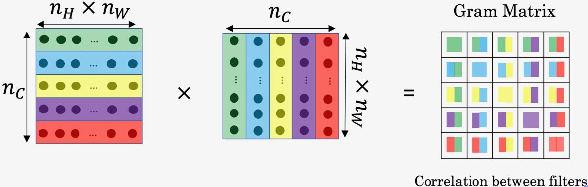
First, we need to know something about the Gram Matrix . In linear algebra, the Gram matrix G of a set of vectors (v1, …, vn) is the matrix of dot products, whose entries are G (i, j) = np.dot(vi, vj) . In other words, G (i, j) compares how similar vi is to vj. If they are highly similar, the outcome would be a large value, otherwise, it would be low suggesting lower correlation. In NST, we can compute the Gram matrix by multiplying the unrolled filter matrix with their transpose as shown below:

The result is a matrix of dimension (nC, nC) where nC is the number of filters. The value G (i, j) measures how similar the activations of filter i are to the activations of filter j. One important part of the gram matrix is that the diagonal elements such as G (i, i) also measures how active filter i is. For example, suppose filter i is detecting vertical textures in the image, then G (i, i) measures how common vertical textures are in the image as a whole.

By capturing the prevalence of different types of features G (i, i), as well as how much different features occur together G (i, j), the Gram matrix G measures the style of an image.

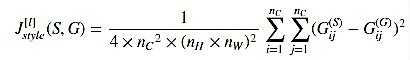
After we have the Gram matrix, we want to minimize the distance between the Gram matrix of the "style" image S and that of the "generated" image G. Usually, we take more than one layers in the account to calculate Style cost as opposed to Content cost (in which only one layer is sufficient), and the reason for doing so is discussed later on in the post. For a single hidden layer, the corresponding style cost is defined as:

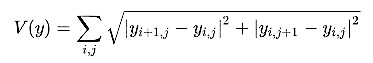
It acts like a regularizer which encourages spatial smoothness in the generated image (G). This was not used in the original paper proposed by [Gatys et al.](https://arxiv.org/pdf/1508.06576.pdf) but it can sometimes improve the results. For 2D signal (or image), it is defined as follows:

What will happen if we zero out the coefficients of the Content and TV loss, assuming we are taking only one layer's activation to compute Style cost?

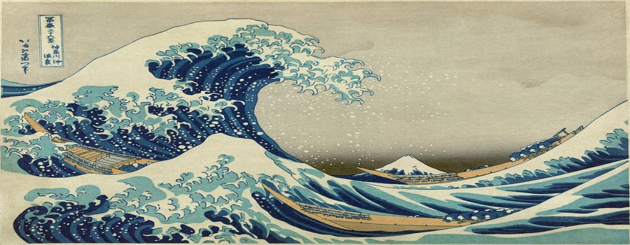
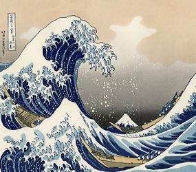
As many of you might have guessed, the optimization algorithm will now only have to minimize the Style cost. So, for a given Style image , we would see what kind of brush-strokes will the model try to enforce in the final generated image (G). Remember, we started with only one layer's activation in the Style cost, so running the experiments for different layers would give different kind of brush-strokes that would be there in the final generated image. Suppose the style image is famous The great wall of Kanagawa shown below:

Here are the brush-strokes that we get after running the experiment taking into account the different layers, one at a time.

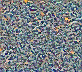
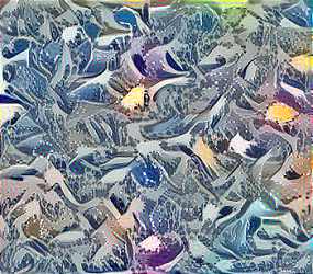
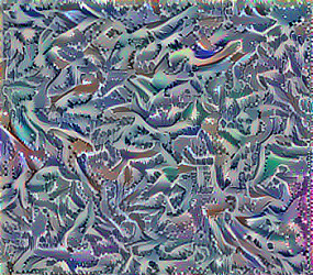
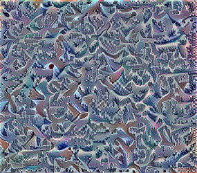
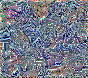
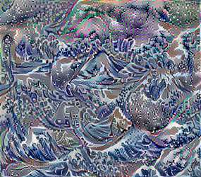
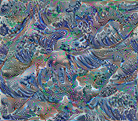
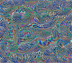
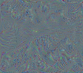
These are brush-strokes that the model learned when layers Conv_2_2, Conv_3_1, Conv_3_2, Conv_3_3, Conv_4_1, Conv_4_3, Conv_4_4, Conv_5_1, and Conv_5_4 (left to right and top to bottom) were used one at a time in the Style cost.

You might be wondering why am I showing these images, what one can conclude after looking at these brush-strokes?

So, the reason behind running this experiment was that - authors of the original paper gave equal weight to the styles learned by different layers while calculating the Total Style Cost (weighted summation of style loss corresponding to different layers). Now, that's not intuitive at all after looking at these images, because we can see that styles learned by the shallower layers are more aesthetically pleasing, compared to what deeper layers learned. So, we would like to assign a lower weight to the deeper layers and higher to the shallower ones; Exponentially decreasing the weights as we go deeper and deeper could be one way.

Similarly, you can run the experiment to minimize only the content cost, and see which layer performs the best (You should always keep in mind that, you only want to transfer the content of the image not exactly copy paste it in the final generated image). I generally find Conv_3_2 to be the best (earlier layers are very good at reconstructing the ditto original image).

The authors investigated Conditional adversarial networks as a general-purpose solution to Image-to-Image Translation problems in this [paper](https://arxiv.org/pdf/1611.07004.pdf). These networks not only learn the mapping from input image to output image, but also learn a loss function to train this mapping. In analogy to automatic language translation, we define automatic image-to-image translation as the task of translating one possible representation of a scene into another, given sufficient training data.

In Generative Adversarial Networks settings, we could specify only a high-level goal, like “make the output indistinguishable from reality”, and then it automatically learn a loss function appropriate for satisfying this goal. Like other GANs, Conditional GANs also have one discriminator (or critic depending on the loss function we are using) and one generator, and it tries to learn a conditional generative model which makes it suitable for Image-to-Image translation tasks, where we condition on an input image and generate a corresponding output image.

If mathematically expressed, CGANs learn a mapping from observed image X and random noise vector z, to y, G : {x, z} → y . The generator G is trained to produce outputs that cannot be distinguished from real images by an adversarially trained discriminator, D, which in turn is itself optimized to do as well as possible at identifying the generator’s fakes.

The figure shown above illustrates the working of GAN in Conditional setting.

The objective of a conditional GAN can be expressed as:

Lc GAN (G, D) = Ex,y (log D(x, y)) + Ex,z (log(1 − D(x, G(x, z)))

, where G tries to minimize this objective against an adversarial D that tries to maximize it, i.e.

G∗ = arg min(G)max(D) Lc GAN (G, D)

It is beneficial to mix the GAN objective with a more traditional loss, such as L1 distance to make sure that, the ground truth and the output are close to each other in L1 sense

L(G) = Ex,y,z ( ||y − G(x, z)|| )

Without z, the net could still learn a mapping from x to y, but would produce deterministic outputs, and therefore would fail to match any distribution other than a delta function . Instead, the authors of Pix2pix provided noise only in the form of dropout , applied on several layers of the generator at both training and test time .

The Min-Max objective mentioned above was used in the original paper when GAN was first proposed by Ian Goodfellow in 2014, but unfortunately, it doesn't perform well due to vanishing gradients problems. Since then, there has been a lot of development, and many researchers have proposed different kinds of loss formulation (LS-GAN, WGAN, WGAN-GP) to overcome these issues. Authors of this paper used Least-square objective function while running their optimization process.

The GAN discriminator models high-frequency structure term, relying on an L1 term to force low-frequency correctness. In order to model high-frequencies, it is sufficient to restrict the attention to the structure in local image patches. Therefore, discriminator architecture was termed PatchGAN – that only penalizes structure at the scale of patches. This discriminator tries to classify if each N × N patch in an image is real or fake. We run this discriminator convolutionally across the image, and average all responses to provide the ultimate output of D. Patch GANs discriminator effectively models the image as a Markov random field, assuming independence between pixels separated by more than a patch diameter. The recpetive field of the discriminator used was 70 * 70 (and was performing best compared to smaller and larger receptive fields).

The 70 × 70 discriminator architecture is: C64 - C128 - C256 - C512

• Alternate between one gradient descent step on D, and one step on G.
• The objective function was divided by 2 while optimizing D, which slows down the rate at which D learns relative to G.
• Use Adam solver, with a learning rate of 2e-4, and momentum parameters β1 = 0.5, β2 = 0.999.
• Use Dropout both at the training and test time.
• Use instance normalization (normalization using the statistics of the test batch) instead of batch normalization.
• Can work even with the much smaller datasets.
• Both L1 and cGAN loss are important to reduce the artifacts in the final output.

Image-to-Image translation is a class of vision and graphics problems where the goal is to learn the mapping between an input image and an output image using a training set of aligned image pairs. However, for many tasks, paired training data will not be available. So, the authors in [this](https://arxiv.org/pdf/1703.10593.pdf) paper presented an approach for learning to translate an image from a source domain X to a target domain Y in the absence of paired examples.

The goal is to learn a mapping G : X → Y such that the distribution of images from G(X) is indistinguishable from the distribution Y using an adversarial loss. Because this mapping is highly under-constrained, they coupled it with an inverse mapping F : Y → X and introduced a cycle consistency loss to enforce F(G(X)) ≈ X (and vice-versa).

Obtaining paired training data can be difficult and expensive. For example, only a couple of datasets exist for tasks like semantic segmentation, and they are relatively small. Obtaining input-output pairs for graphics tasks like artistic stylization can be even more difficult since the desired output is highly complex, typically requiring artistic authoring. For many tasks, like object transfiguration (e.g., zebra <-> horse), the desired output is not even well-defined. Therefore, the authors tried to present an algorithm that can learn to translate between domains without paired input-output examples. The primary assumption is that there exists some underlying relationship between the domains. Although there is a lack of supervision in the form of paired examples, supervision at the level of sets can still be exploited: one set of images in domain X and a different set in domain Y.

The optimal G thereby translates the domain X to a domain Y distributed identically to Y. However, such a translation does not guarantee that an individual input x and output y are paired up in a meaningful way – there are infinitely many mappings G that will induce the same distribution over y . Key points:

• Difficult to optimize adversarial objective in isolation - standard procedures often lead to the well-known problem of mode collapse.

• Exploited the property that translation should be Cycle consistent . Mathematically, translator G : X → Y and another translator F : Y → X, should be inverses of each other (and both mappings should be bijections).

• Enforcing the structural assumption by training both the mapping G and F simultaneously, and adding a cycle consistency loss that encourages F(G(x)) ≈ x and G(F(y)) ≈ y

  .

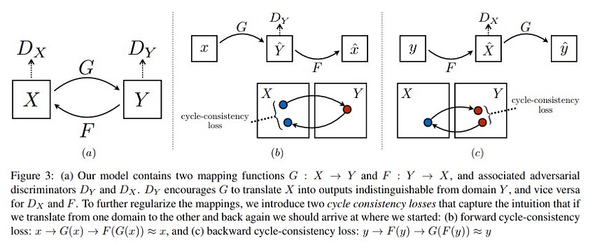
As illustrated in figure, their model includes two mappings G : X → Y and F : Y → X. In addition, they introduced two adversarial discriminators DX and DY , where DX aims to distinguish between images {x} and translated images {F(y)}; in the same way, DY aims to discriminate between {y} and {G(x)}. So, final objective contains two types of terms: adversarial losses for matching the distribution of generated images to the data distribution in the target domain; and cycle consistency losses to prevent the learned mappings G and F from contradicting each other.

Adversarial loss is applied to both mapping functions - G : X → Y and its discriminator DY and F : Y → X and its discriminator DX, where G tries to generate images G(x) that look similar to images from domain Y , while DY aims to distinguish between translated samples G(x) and real samples y (similar condition holds for the other one).

• Generator (G) tries to minimize E[x∼pdata(x)] (D(G(x)) − 1)** 2
• Discriminator (DY) tries to minimize E[y∼pdata(y)] (D(y) − 1)**2 + E[x∼pdata(x)] D(G(x))**2
• Generator (F) tries to minimize E[y∼pdata(y)] (D(G(y)) − 1)** 2
• Discriminator (DX) tries to minimize E[x∼pdata(x)] (D(x) − 1)**2 + E[y∼pdata(y)] D(G(y))**2

Adversarial training can, in theory, learn mappings G and F that produce outputs identically distributed as target domains Y and X respectively (strictly speaking, this requires G and F to be stochastic functions). However, with large enough capacity, a network can map the same set of input images to any random permutation of images in the target domain, where any of the learned mappings can induce an output distribution that matches the target distribution. Thus, adversarial losses alone cannot guarantee that the learned function can map an individual input xi to a desired output yi. To further reduce the space of possible mapping functions, learned functions should be cycle-consistent.

Lcyc (G, F) = E[x∼pdata(x)] || F(G(x)) − x|| + E[y∼pdata(y)] || G(F(y)) − y || 

The full objective is:

L (G, F, DX, DY) = LGAN (G, DY , X, Y) + LGAN (F, DX, Y, X) + λLcyc(G, F)

, where lambda controls the relative importance of the two objectives.

• This model can be viewed as training two autoencoders: first F◦G : X → X jointly with second G◦F : Y → Y.

• These have special internal structures - map an image to itself via an intermediate representation that is a translation of the image into another domain.

• Can also be seen as a special case of adversarial autoencoders , which use an adversarial loss to train the bottleneck layer of an autoencoder to match an arbitrary target distribution.

• The target distribution for the X → X autoencoder is the domain Y and for the Y → Y autoencoder is the domain X.

• Two stride-2 convolutions, several residual blocks, and two fractionally strided convolutions with stride 1/2.
• 6 blocks for 128 × 128 images and 9 blocks for 256 × 256 and higher resolution training images.
• Instance normalization instead of batch normalization.

• Patch Discriminator - 70 × 70 PatchGANs, which aim to classify whether 70 × 70 overlapping image patches are real or fake (more parameter efficient compared to full-image discriminator)

• To reduce model oscillation, update the discriminators using a history of generated images rather than the latest ones - always keep an image buffer of 50 previously generated images.

• Set λ to 10 in total loss equation, use the Adam solver with a batch size of 1
• Learning rate of 0.0002 for the first 100 epochs and then linearly decay the rate to zero over the next 100 epochs.

Generator:
- Network with 6 residual blocks: c7s1-64, d128, d256, R256, R256, R256, R256, R256, R256, u128, u64, c7s1-3
- Network with 9 residual blocks: c7s1-64, d128, d256, R256, R256, R256, R256, R256, R256, R256, R256, R256, u128, u64, c7s1-3

Discriminator:
- C64-C128-C256-C512

c7s1-k denote a 7×7 Convolution-InstanceNormReLU Layer with k filters and stride 1. dk denotes a 3 × 3 Convolution-InstanceNorm-ReLU layer with k filters and stride 2. Reflection padding was used to reduce artifacts. Rk denotes a residual block that contains two 3 × 3 convolutional layers with the same number of filters on both layer. uk denotes a 3 × 3 fractional-strided-ConvolutionInstanceNorm-ReLU layer with k filters and stride 1/2. Ck denote a 4 × 4 Convolution-InstanceNorm-LeakyReLU layer with k filters and stride 2. After the last layer, a convolution is applied to produce a 1-dimensional output. **Do not** use InstanceNorm for the first C64 layer. Use leaky ReLUs with a slope of 0.2

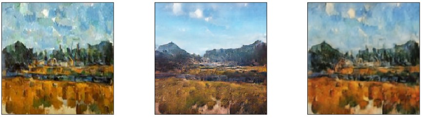
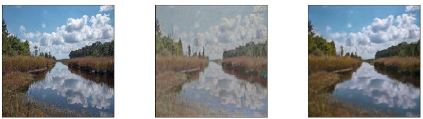
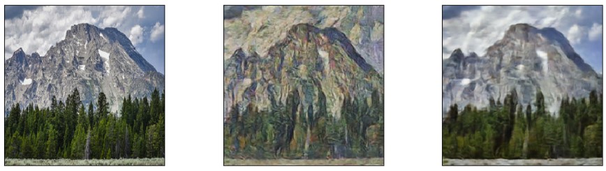
For painting → photo, they found that it was helpful to introduce an additional loss to encourage the mapping to preserve color composition between the input and output. In particular, they regularized the generator to be near an identity mapping when real samples of the target domain are provided as the input to the generator i.e.,

Lidentity (G, F) = E[y∼pdata(y)] || G(y) − y || + E[x∼pdata(x)] || F(x) − x ||

Thanks for going through this post! Any feedbacks are duly appreciated.