Self-Driving Car Engineer Nanodegree

Deep Learning

Project: Build a Traffic Sign Recognition Classifier

Step 1: Dataset Summary

The pickled data is a dictionary with 4 key/value pairs:

'features' is a 4D array containing raw pixel data of the traffic sign images, (num examples, width, height, channels).
'labels' is a 1D array containing the label/class id of the traffic sign. The file signnames.csv contains id -> name mappings for each id.
'sizes' is a list containing tuples, (width, height) representing the original width and height the image.
'coords' is a list containing tuples, (x1, y1, x2, y2) representing coordinates of a bounding box around the sign in the image. THESE COORDINATES ASSUME THE ORIGINAL IMAGE. THE PICKLED DATA CONTAINS RESIZED VERSIONS (32 by 32) OF THESE IMAGES

Complete the basic data summary below. Use python, numpy and/or pandas methods to calculate the data summary rather than hard coding the results. For example, the pandas shape method might be useful for calculating some of the summary results.

Provide a Basic Summary of the Data Set Using Python, Numpy and/or Pandas


    Number of training examples = 34799
    Number of testing examples = 12630
    Image data shape = (32, 32, 3)
    Number of classes = 43

Step 2: Exploratory Visualization

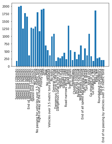
Visualize the German Traffic Signs Dataset using the pickled file(s). This is open ended, suggestions include: plotting traffic sign images, plotting the count of each sign, etc.

The following figure shows the data visualization with the labels on X-axis

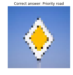
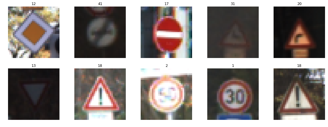
Here are few example training data

Step 3: Preprocessiong

Minimally, the image data should be normalized so that the data has mean zero and equal variance. For image data, (pixel - 128)/ 128 is a quick way to approximately normalize the data and can be used in this project.

Other pre-processing steps are optional. You can try different techniques to see if it improves performance.

Use the code cell (or multiple code cells, if necessary) to implement the first step of your project.

In this code the image data is converted to grayscale and normalized.Converting the images to grayscale reduces the computation time by reducing the parameters.

### Preprocess the data here. It is required to normalize the data. Other preprocessing steps could include 
### converting to grayscale, etc.
### Feel free to use as many code cells as needed.
from sklearn.utils import shuffle

X_train=np.sum(X_train_rgb/3, axis=3, keepdims=True)
X_test=np.sum(X_test_rgb/3, axis=3, keepdims=True)
X_valid=np.sum(X_valid_rgb/3, axis=3, keepdims=True)
X_train=(X_train - 128)/128
X_test=(X_test - 128)/128
X_train,y_train=shuffle(X_train,y_train)

Step 4: Model Architecture

Layer	Description
Input	32x32x1 grayscale image
Convolution 5x5	2x2 stride, valid padding, outputs 28x28x6
RELU
Max pooling	2x2 stride, outputs 14x14x6
Convolution 5x5	2x2 stride, valid padding, outputs 10x10x16
RELU
Max pooling	2x2 stride, outputs 5x5x16
Convolution 1x1	2x2 stride, valid padding, outputs 1x1x400
RELU
Fully connected	input 400, output 120
RELU
Dropout	50% keep
Fully connected	input 120, output 84
RELU
Dropout	50% keep
Fully connected	input 84, output 43

Step 5: Model Training

A validation set can be used to assess how well the model is performing. A low accuracy on the training and validation sets imply underfitting. A high accuracy on the training set but low accuracy on the validation set implies overfitting.

While training AdamOptimizer was used. Total number of 30 epochs were used as it resulted with optimal result.

The batch size of 150 was fixed. The learning rate was set to 0.00097. Lowering the learning rate than this value resulted in bad validation accuracy.

from tensorflow.python.client import device_lib 
print(device_lib.list_local_devices())

[name: "/device:CPU:0"
device_type: "CPU"
memory_limit: 268435456
locality {
}
incarnation: 4563718365486527491
, name: "/device:GPU:0"
device_type: "GPU"
memory_limit: 3162085785
locality {
  bus_id: 1
  links {
  }
}
incarnation: 6800002227496049498
physical_device_desc: "device: 0, name: GeForce GTX 1050 Ti, pci bus id: 0000:01:00.0, compute capability: 6.1"
]

Step 6: Solution Approach

The following is the training process output


    Training...
    
    EPOCH 1 ...
    Training Accuracy = 0.703
    Validation Accuracy = 0.651
    
    EPOCH 2 ...
    Training Accuracy = 0.883
    Validation Accuracy = 0.822
    
    EPOCH 3 ...
    Training Accuracy = 0.931
    Validation Accuracy = 0.867
    
    EPOCH 4 ...
    Training Accuracy = 0.946
    Validation Accuracy = 0.895
    
    EPOCH 5 ...
    Training Accuracy = 0.964
    Validation Accuracy = 0.889
    
    EPOCH 6 ...
    Training Accuracy = 0.974
    Validation Accuracy = 0.918
    
    EPOCH 7 ...
    Training Accuracy = 0.984
    Validation Accuracy = 0.934
    
    EPOCH 8 ...
    Training Accuracy = 0.988
    Validation Accuracy = 0.933
    
    EPOCH 9 ...
    Training Accuracy = 0.985
    Validation Accuracy = 0.934
    
    EPOCH 10 ...
    Training Accuracy = 0.992
    Validation Accuracy = 0.926
    
    EPOCH 11 ...
    Training Accuracy = 0.993
    Validation Accuracy = 0.934
    
    EPOCH 12 ...
    Training Accuracy = 0.993
    Validation Accuracy = 0.925
    
    EPOCH 13 ...
    Training Accuracy = 0.996
    Validation Accuracy = 0.938
    
    EPOCH 14 ...
    Training Accuracy = 0.996
    Validation Accuracy = 0.941
    
    EPOCH 15 ...
    Training Accuracy = 0.993
    Validation Accuracy = 0.927
    
    EPOCH 16 ...
    Training Accuracy = 0.997
    Validation Accuracy = 0.942
    
    EPOCH 17 ...
    Training Accuracy = 0.998
    Validation Accuracy = 0.946
    
    EPOCH 18 ...
    Training Accuracy = 0.997
    Validation Accuracy = 0.944
    
    EPOCH 19 ...
    Training Accuracy = 0.997
    Validation Accuracy = 0.937
    
    EPOCH 20 ...
    Training Accuracy = 0.999
    Validation Accuracy = 0.945
    
    EPOCH 21 ...
    Training Accuracy = 0.998
    Validation Accuracy = 0.943
    
    EPOCH 22 ...
    Training Accuracy = 0.998
    Validation Accuracy = 0.939
    
    EPOCH 23 ...
    Training Accuracy = 0.999
    Validation Accuracy = 0.947
    
    EPOCH 24 ...
    Training Accuracy = 1.000
    Validation Accuracy = 0.946
    
    EPOCH 25 ...
    Training Accuracy = 0.999
    Validation Accuracy = 0.951
    
    EPOCH 26 ...
    Training Accuracy = 0.998
    Validation Accuracy = 0.939
    
    EPOCH 27 ...
    Training Accuracy = 0.997
    Validation Accuracy = 0.949
    
    EPOCH 28 ...
    Training Accuracy = 0.999
    Validation Accuracy = 0.946
    
    EPOCH 29 ...
    Training Accuracy = 1.000
    Validation Accuracy = 0.946
    
    EPOCH 30 ...
    Training Accuracy = 1.000
    Validation Accuracy = 0.949
    
    Model saved

plt.plot(validation_accuracy_figure)
plt.title("Test Accuracy")
plt.show()

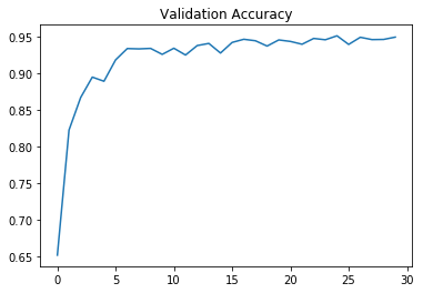
plt.plot(validation_accuracy_figure)
plt.title("Validation Accuracy")
plt.show()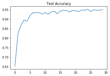

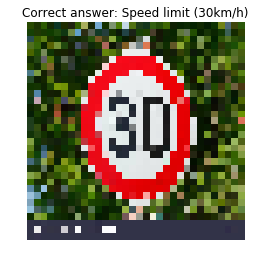
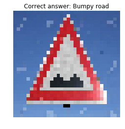
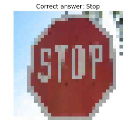
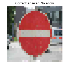
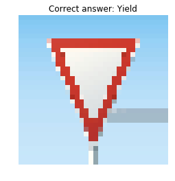
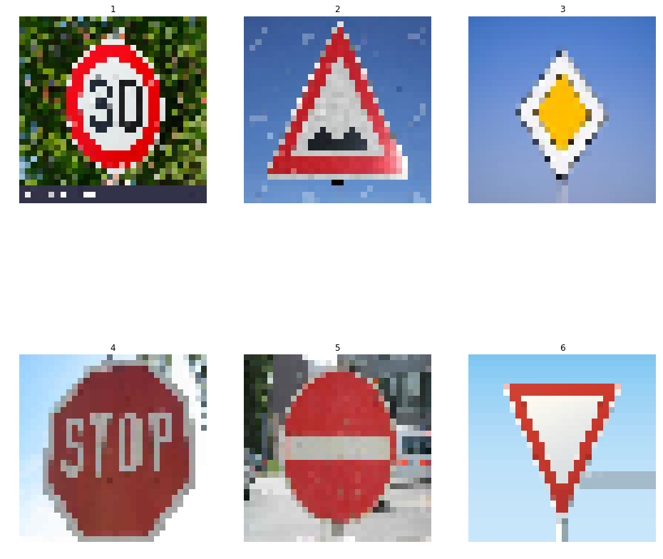
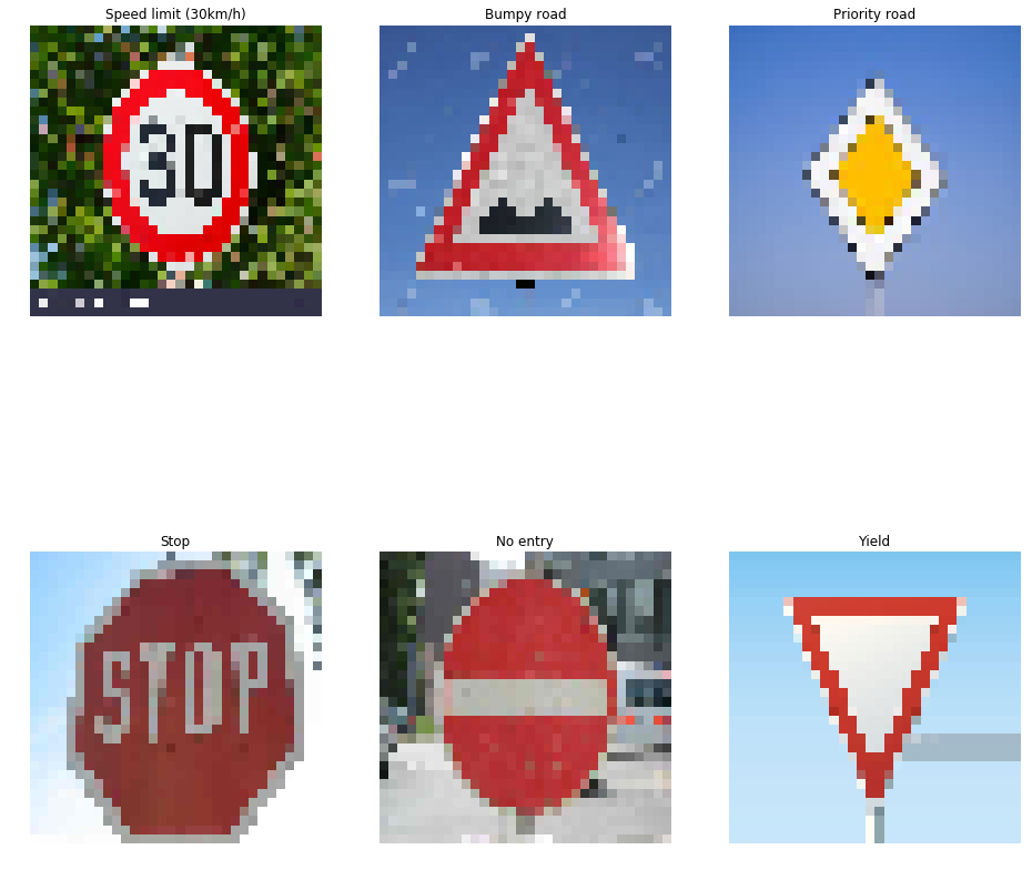
Step 7: Accuring new images

Six new images are accured from Google images as shown

Step 8: Performance on new images

test_data=np.uint8(np.zeros((6,32,32,3)))
for i in range(num_test_img):
    test_data[i] = test_img[i]
test_data=np.sum(test_data/3, axis=3, keepdims=True)
test_data=(test_data - 128)/128
with tf.Session() as sess:
    saver.restore(sess,'./lenet.ckpt')
    signs_classes=sess.run(tf.arg_max(logits,1),feed_dict={x:test_data,keep_prob:1.0})
    
figsize=(16,16)
plt.figure(figsize=figsize)
for i in range(num_test_img):
    plt.subplot(2,3,i+1)
    plt.imshow(test_img[i])
    plt.title(signs_names[signs_classes[i]])
    plt.axis('off')
    
plt.show()

INFO:tensorflow:Restoring parameters from ./lenet.ckpt

Analyze Performance

### Calculate the accuracy for these 5 new images. 
### For example, if the model predicted 1 out of 5 signs correctly, it's 20% accurate on these new images.
correct_class=[1,22,12,14,17,13]
correct=0
for (corr,pred) in zip(correct_class,signs_classes):
    if corr==pred:
        correct+=1
        
print("Accuracy: ",round(correct/6,3))

Accuracy:  1.0

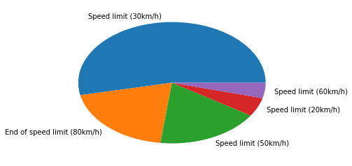
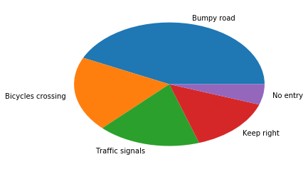
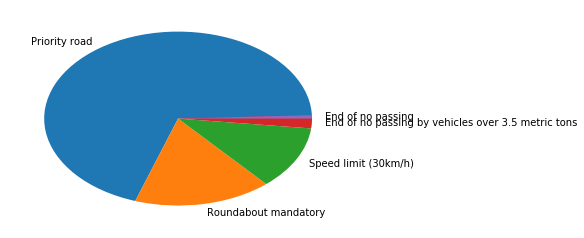
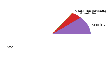
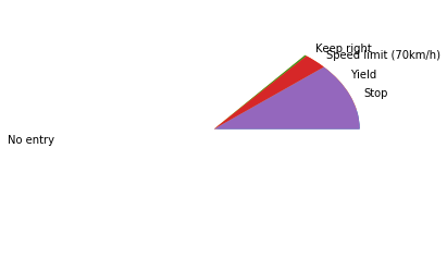
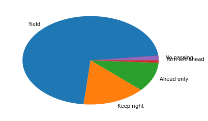
Step 9: Model Certainty - Softmax Probabilities

The top five softmax probabilities of the predictions on the captured images are outputted. The submission discusses how certain or uncertain the model is of its predictions.