This project is about using machine learning algorithms to predict whether or not a student would pass the final exam. The data set used is from UCI Machine Learning Repository.
National institute of posts and telecommunications INPT Rabat, Morocco.
Education is an important element of the society, every government and country in the world work so hard to improve this sector. With the corona-virus outbreak that has disrupted life around the globe in 2020, the educational systems have been affected in many ways; studies show that student’s performance has decreased since then, which highlights the need to deal with this problem more seriously and try to find effective solutions, as well as the influencing factors.
The educational systems need, at this specific time, innovative ways to improve quality of education to achieve the best results and decrease the failure rate.
As students of the IT department who studied in the last month a little about machine learning, we know that in order for an institute to provide quality education to learners, deep analysis of previous records of the learners can play a vital role, and wanted to work on this challenging task.
As already mentioned, with the help of the old students records, we can came up with a model that can let us help students improve their performance in exams by predicting the student success. So, it is obvious it's a problem of classification , and we will classify a student based on his given informations, and we will also use diffrent classifiers such as KNN or SVM classifier and compare between them. Many factors affect a student performance in exams like famiily problems or alcohol consumption, and by using our skills in machine learning we want to :
    1) predict whether a student will pass his final exam or not.
    2) came up with the best classifier that is more accurate and avoid
    overfitting and underfitting by using simple techniques.
    3) know what the most factors affect a student performance.
So, teachers and parents will be able to intervene before students reach the exam stage and solve the problems.
Now before training our model we have to process our data :
-
We have to map each string to a numerical value so that it can be used for model training.
Let's take an example to make this clear : The mother job column contain five values : 'teacher',
'health','services', 'at_home' and 'other'.

Our job then is to map each of these string to numerical values, and this is how it's done :
df['Mjob'] = df['Mjob'].map({'teacher': 0, 'health': 1, 'services': 2, 'at_home': 3, 'other': 4})
-
We have to perform feature scaling :
 	Feature scaling is a method used to normalize the range of independent variables
 or features of data. In data processing, it is also known as data normalization
 and is generally performed during the data preprocessing step.

 This will allow our learning algorithms to converge very quickly. The operation requires
 to take each column, let's say 'col', and replace it by :
But this is not the only scaling you can do, you can try also :, where std refers to standard deviation.
After having our dataset processed, we move to the next step which is dataset visualization; so that patterns, trends and correlations that might not otherwise be detected can be now exposed.
This discipline will give us some insights into our data and help us understand the dataset by placing it in a visual context using python libraries such as: matplotlib and seaborn.
There are so many ways to visualize a dataset. In this project we chose to:
  #1- Plot distribution histograms so that we can see the number of samples that occur in
  each specific category.
  E.g.  Internet accessibility at home distribution shows that our dataset consists of
  more than 300 students with home internet accessibility,
  while there are about 50 students who have no access to the internet at home.

  #2- Plot “Boxplots” to see to see how the students status is distributed according to each variable.

  #3- Plot the correlation output that should list all the features and their correlations
  to the target variable.
  So that we have an idea about the most impactful elements on the students status.
Before starting training our classifers let us define the metrics that we will use to compare between our three classifiers :
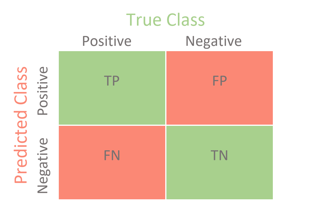
1) Confusion matrix :
2) F1 score :

TP = number of true positives
FP = number of false positives
FN = number of false negatives
3) The roc curve : A receiver operating characteristic curve, or ROC curve,
is a graphical plot that illustrates the diagnostic ability of a binary
classifier system as its discrimination threshold is varied.

4) ROC score : it's simply the value of the area under the roc curve.
The best value is 1 because the area of 1x1 square is 1.
Now let's start by the first learning algorithm :
1)Introduction to knn :
K-Nearest Neighbour is one of the simplest Machine Learning algorithms based on Supervised Learning technique.Its assumes the similarity between the new case data and available cases and put the new case into the category that is most similar to the available categories.K-NN algorithm stores all the available data and classifies a new data point based on the similarity. This means when new data appears then it can be easily classified into a well suite category by using K- NN algorithm.
2)Advantages and Disadvantages of Knn algorithm:
2.1Advantages:
-It is simple to implement.
-It is robust to the noisy training data
-It can be more effective if the training data is large.
2.2Disadvantages
-Always needs to determine the value of K which may be complex some time.
-The computation cost is high because of calculating the distance between all training set
3)How does it work :
The K-NN working can be explained on the basis of the below Algorithm:
Step-1: Select the number K of the neighbors
Step-2: Calculate the Euclidean(or any other type of distances) distance of K number of neighbors
Step-3: Among the k nearest neighbors, count the number of the data points in each category.
Step-4: Assign the new data points to that category for which the number of the neighbor is maximum.
Suppose we have a new data point and we need to put it in the required category. Consider the below image:
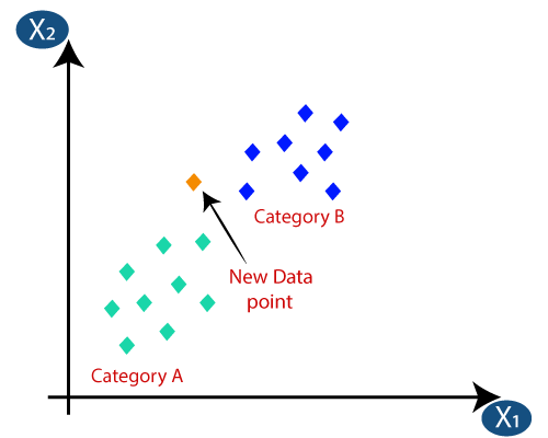
-Firstly, we will choose the number of neighbors, so we will choose the k=5.
-Next, we will calculate the Euclidean distance between the data points
-By calculating the Euclidean distance we got the nearest neighbors,
as three nearest neighbors in category A and two nearest neighbors in category B.
Consider the image below:
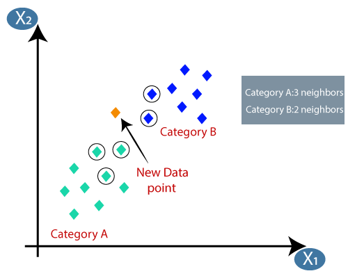
As we can see the 3 nearest neighbors are from category A, hence this new data point must belong to category A.
4)Python implementation of the KNN algorithm
In this step we will implement knn for our case study by following this step:
a) Data preprocessing step
b) Hyperparameters tuning
c) Fitting the K-NN algorithm to the Training set
d) Predicting the test result
e) Test accuracy of the result
*Let's look into each step separately
a) Data preprocessing step:
we should look into previous section
b) Hyperparameters tuning:
In this step we look after 2 methods to tune the best parameters for our model
_First method:
tuning the best k for better test_acquracy and training_acquracy using k-NN Varying number of neighbors plot

-Second method:
In this method we search for the Best parameters(K,metric=Distance) based on time and accuracy

c,d) Fitting and predicting
*After finding the best parameters with high accuracy we fit the model to training_set and predicting the result using test_set

e) Test accuracy of the result
*After prediction we will evaluate the model using various methods:
1) Confusion_matrix:

2) Classification_report :

3) Ploting Roc curv:

f) Conclusion of the work:

Now we will use Support Vector Machine algorithm and see how it will act on our data. But, let's define what is svm algorithm
In machine learning, support-vector machines are supervised learning models with
associated learning algorithms that analyze data for classification
and regression analysis.
It uses a technique called the kernel trick to transform your data and then based on these transformations it finds an optimal boundary between the possible outputs. We will use three kernel : Linear, polynomial and gaussian kernel.
1) Linear kernel : Linear Kernel is used when the data is Linearly separable, that is,
it can be separated using a single Line. It is one of the most common kernels to be used.
It is mostly used when there are a Large number of features in a particular Data Set.

2)  the polynomial kernel is a kernel function commonly used with support vector machines and
other kernelized models, that represents the similarity of vectors in a feature space over
polynomials of the original variables, allowing learning of non-linear models.

3) Gaussian RBF(Radial Basis Function) is another popular Kernel method used in SVM models for more.
RBF kernel is a function whose value depends on the distance from the origin or from some point.
Gaussian Kernel is of the following format:
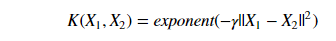
Using the distance in the original space we calculate the dot product (similarity) of X1 & X2.
Note: similarity is the angular distance between two points.
Here are some plots for the three kernels that we've talked about :

Now after we train our three models, here are the metrics and the ROC plots for each svm kernel :
But let's talk about some parameters that are using in SVM :
-
: The C parameter tells the SVM optimization how much you want to avoid misclassifying each training example.
-
: It's basically the degree of the polynomial used to find the hyperplane to split the data.
-
: Intuitively, the gamma parameter defines how far the influence of a single training example reaches, with low values meaning ‘far’ and high values meaning ‘close’. The gamma parameters can be seen as the inverse of the radius of influence of samples selected by the model as support vectors.
on the cross validation set.
So here is how it will be done:
Repeat{
- choose c
- Train the svm model
- calculate
}
After that we will be able to get the optimal value of c.
1) Linear kernel : svm.svc(C)
After training our first svm model, here are our results :
| Metric | Value |
|---|---|
| training time | 10ms |
| accuracy | 84.0 % |
| f1 score | 0.82 |
| The roc_auc_score | 0.8 |
Confusion matrix :

ROC Curve :

2) Polynomial kernel : svm.svc(C,d)
Here we will use diffrent values for both C and d. For example if we have 2 values for C and 3 values for d then we have 2x3 possibilities.
After training our second svm model, here are our results :
| Metric | Value |
|---|---|
| training time | 7ms |
| accuracy | 78.00 % |
| f1 score | 0.74 |
| The roc_auc_score | 0.73 |
Confusion matrix :

ROC Curve :

3) Gaussian kernel : svm.svc(C,gamma)
Here we will use diffrent values for both C and gamma.
After training our last svm model, here are our results :
| Metric | Value |
|---|---|
| training time | 16ms |
| accuracy | 83.0 % |
| f1 score | 0.77 |
| The roc_auc_score | 0.74 |
Confusion matrix :

ROC Curve :

Now, after training our three svm models, it is better to group all the results so it can be easy to compare between them :
Now after we train our three models, here are the metrics and the ROC plots :
This table contains all metrics :
| Metric | Linear kernel | polynomial kernel | gaussian kernel |
|---|---|---|---|
| training time | 11ms | 7ms | 3ms |
| accuracy % | 84.375 | 78.125 | 82.8125 |
| confusion matrix | [15 8] [2 39 |
[12 8] [6 38] |
[10 11] [0 43] |
| f1 score | 0.82 | 0.74 | 0.77 |
| roc_auc_score | 0.80 | 0.73 | 0.74 |

As you can see the training times are soo small thanks to feature scaling. As you can also notice, the best svm model the one that used the linear kernel. So let's show the results of this linear kernel svm model again :
The training time : 11ms
The accuracy : 84.375 %
The f1 score : 0.82
The roc_auc_score : 0.8
The roc curve :

As you can see the accuracy is pretty good for our problem, but we need to see also
that the f1 score has a high value so the model performed very well on the test set.
Our model is able to generlize for new data and get good prediction.
The value of the area under the roc curve is approximatly 0.80 which is good,
this tells us that the model is capable of distinguishing between the two classes.
After validating our model, lets extract the positive and negative factors, in the iPython notebook we explained very well how we managed to do that :
After calling the appropriate function, we got:
Factors helping students succeed :
father's education
guardian
wants to take higher education
studytime
father's job
Factors leading students to failure :
age
health
going out with friends
absences
failures
Conclusion :
-
1) For positive impact, it seems that the factors helping students succeed:
- Father's education : if the father has a higher education, he will help his children in their studies so that they will not struggle for a long time with their homeworks.

- Guardian : This instance takes three values as our convention: 0,1 and 2, 2 refers to 'other', we conclude than if the guardian is neither mother nor father than the student has a big chance to succeed, but this just the result of our classifer, it is difficult to judge that.

- Wants to take higher education : Students who are looking forward to take higher education seems to be motivated and having goals to achieve.

- Study time : This is an import thing to keep in mind, students need to spend many hours studying, do not imagine a student succeeding in his exams and yet do not spend one hour at his desk, but it depends on many things such as subject, timetable ...

- Father's job : If the father has a good career, then of course he will fulfill the needs of their children in terms of paying additive classes, internet ...

-
2) For negative impact, it seems that the factors affecting students are:
- Age : It is difficult to judge that the age is a negative factor, we do not have a big dataset to generalize, but we will assume it's a negative factor for the two choosen portuguese schools, so students should go to high school early.

- Health : This can not be taken into consideration, we cannot say that students having good health fail in the exams, but we will assume again it's a negative factor for the two choosen portuguese schools as our classifier told us.

- Going out with friends : going out with friends helps relieve stress, but sometimes if the students spend a lot of time outside the home this will definitely affect their studies.

- Absences : Students who missed classes will find it difficult to take the exams, sometimes you find students read a one month course in just one day, imagine how those students prepare for exams. Now, we did not talk about the students having problems letting them do that, we will later on talk abou that.

- Failures : Having a lot of failures is an indication of a lack of good exam preparations.

- For positive impacts the classifier managed to give reasonable factors except the guardian factor, but if we see the negative factors, one or maybe two of them seems to be not right, Age and Health, I think Health isn't quit good factor to take into consideration if we want to generalize, but as we've said before we will assume that those are a negative factors, but we can say also it is a problem of lack of informations, 395 instances isn't quit big that much, we will assume that is convenient for the two chosen school, but if we see other factors it is indeed a good results.
Now, based on extracted factors, let's give some advices for students, parents and school administration :
- People should get educated especially men so that they help their children in their studies.
- The government should help students whose parents are not rich that much so they get access to internet or looking forward taking higher education.
- Administration should send warnings to parents when students reach the maximum acceptable number of absences before exam period begin.
- When students are having a lot of failures, the administration, teachers should search for the problems faced by this students and also get contact with the parents for more informations.
- Student should find, at home, a suitable space to study, they need desks or just a small area when they can focus on their studies. Imagine how you would tell this student not to go out with his friends and spend a lot of time and yet their parents shout all the time in front of him. Parents should keep their problems for themselves. These students need love and peace at home. Students will then spend many hours studying at home.
Improving the education system is a big problem, as an engineering student we can help achieve this goal by using technologies and study resources like machine learning materials, to come up with an innovative solution to help the student in need, especially students who live in difficult conditions. conditions (demographic, social and educational issues). In this project, we came up with the idea of creating a model that predicts the status of students based on different functionalities. Our main challenges were to define the best classification algorithm and identify the most influential factors for the academic status of students to provide them with a summary or valedictorian of the best conditions for students to achieve high academic status and avoid failures. For this project entitled “Prediction of student performance and difficulty” ”, we used several classification methods such as logistic regression, KNN and SVM and we evaluate this model using different metrics like f1 score, roc curve and the confusion matrix and finally we got a winner with SVM with a precision of 80%compared to other algorithm . Before taking up our main challenges, there were several steps to take: -data processing -data visualization -Implementation of models -comparison of 3 algorithms