![]()
PyCurve is a Python package that provides to user high level yield curve usefull tool. For example you can istanciate a Curve and get a d_rate, a discount factor, even forward d_rate given multiple methodology from Linear Interpolation to parametrization methods as Nelson Siegel or Bjork-Christenssen. PyCurve is also able to provide solutions in order to build yield curve or price Interest rates derivatives via Vasicek or Hull and White.
Below this is the features that this package tackle :
- Curve Smoothing:
- Create Curve Object with two numpy array (t,rt)
- Linear interpolation given a Curve
- Cubic interpolation given a Curve
- Nelson Siegel and Svensson model creation and components plotting
- Nelson Siegel and Svensson calibration given a Curve
- Bjork Christensen and Augmented (6 factors) model creation and components plotting
- Stochastic Modelling:
- Vasicek Model Simulation
- Hull and White one factor Model Simulation
From pypi
pip install PyCurveFrom pypi specific version
pip install PyCurve==0.0.5From Git
git clone https://github.com/ahgperrin/PyCurve.git
pip install -e . This object consists in a simple yield curve encapsulation. This object is used by others class to encapsulate results or in order to directly create a curve with data obbserved in the market.
| Attributes | Type | Description |
|---|---|---|
| rt | Private | Interest rates as float in a numpy.ndarray |
| t | Private | Time as float or int in a numpy.ndarray |
| Methods | Type | Description | Return |
|---|---|---|---|
| get_rate | Public | rt getter | _rt |
| get_time | Public | rt getter | _t |
| set_rate | Public | rt getter | None |
| set_time | Public | rt getter | None |
| is_valid_attr(attr) | Private | Check attributes validity | attribute |
| plot_curve() | Public | Plot Yield curve | None |
from PyCurve.curve import Curve
time = np.array([0.25, 0.5, 0.75, 1., 2.,
        3., 4., 5., 10., 15.,
        20.,25.,30.])
rate = np.array([-0.63171, -0.650322, -0.664493, -0.674608, -0.681294,
        -0.647593, -0.587828, -0.51251, -0.101804,  0.182851,
        0.32962,0.392117,  0.412151])
curve = Curve(rate,time)
curve.plot_curve()
print(curve.get_rate)
print(curve.get_time)
[ 0.25 0.5 0.75 1. 2. 3. 4. 5. 10. 15. 20. 25.
30. ]
[-0.63171 -0.650322 -0.664493 -0.674608 -0.681294 -0.647593 -0.587828
-0.51251 -0.101804 0.182851 0.32962 0.392117 0.412151]

This object consists in a simple simulation encapsulation. This object is used by others class to encapsulate results of monte carlo simulation. This Object has build in method that could perform the conversion from a simulation to a yield curve or to a discount factor curve.
| Attributes | Type | Description |
|---|---|---|
| sim | Private | Simulated paths matrix numpy.ndarray |
| dt | Private | delta_time as float or int in a numpy.ndarray |
| Methods | Type | Description & Params | Return |
|---|---|---|---|
| get_sim | Public | sim getter | _rt |
| get_nb_sim | Public | nb_sim getter | sim.shape[0] |
| get_steps | Public | steps getter | sim.shape[1] |
| get_dt | Public | dt getter | _dt |
| is_valid_attr(attr) | Private | Check attributes validity | attribute |
| yield_curve() | Public | Create a yield curve from simulated paths | Curve |
| discount_factor() | Public | Convert d_rate simulation to discount factor | np.ndarray |
| plot_discount_curve(average) | Public | Plot discount factor (average :bool False plot all paths True Plot estimate) | None |
| plot_simulation() | Public | Plot Yield curve | None |
| plot_yield_curve() | Public | Plot Yield curve | None |
| plot_model() | Public | Plot Yield curve | None |
Using Vasicek to Simulate
from PyCurve.vasicek import Vasicek
vasicek_model = Vasicek(0.02, 0.04, 0.001, -0.004, 50, 30 / 365)
simulation = vasicek_model.simulate_paths(2000) #Return a Simulation and then we can apply Simulation Methods
simulation.plot_yield_curve()
simulation.plot_model()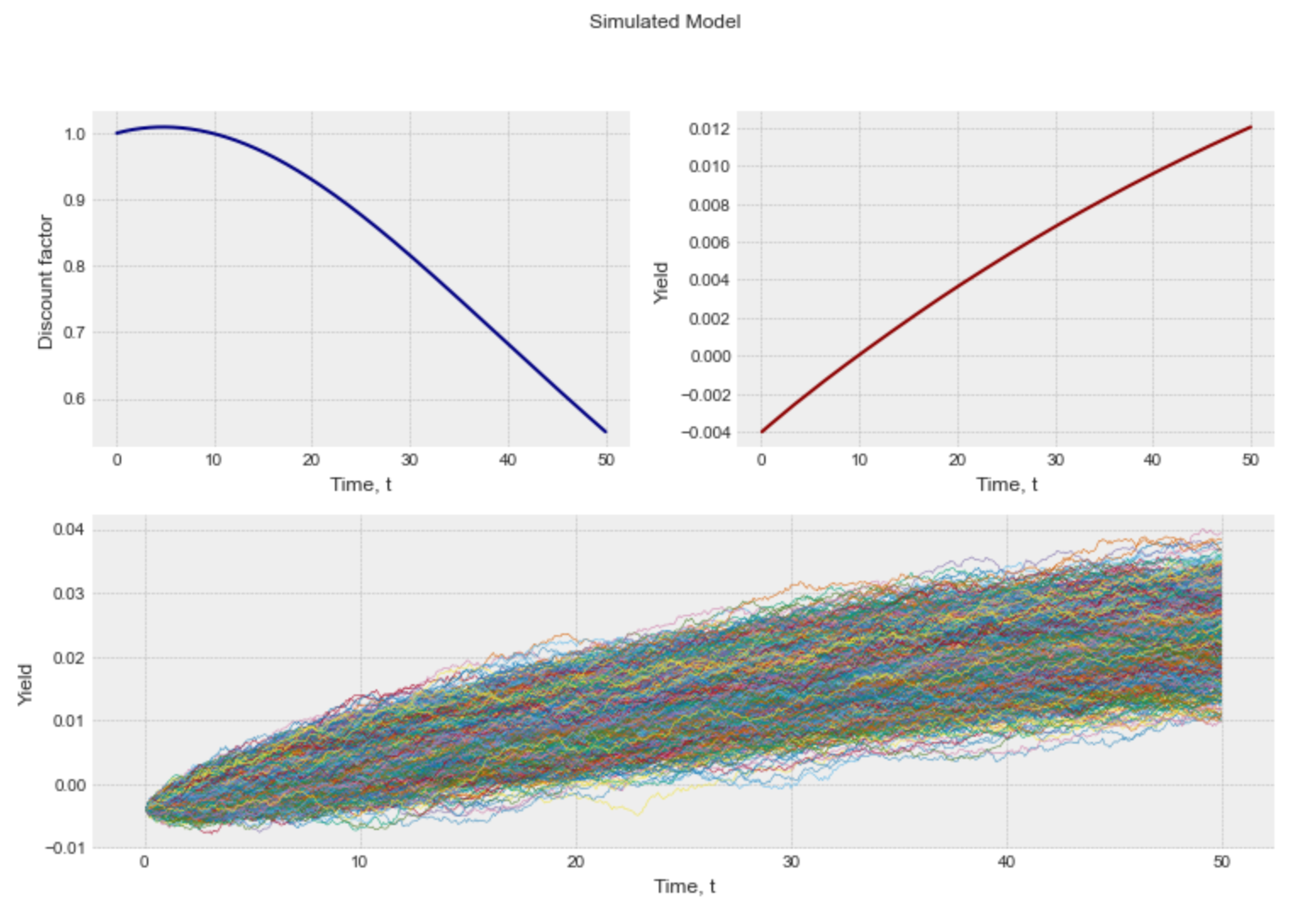
This section is the description with examples of what you can do with this package Please note that for all the examples in this section curve is referring to the curve below you can see example regarding Curve Object in the dedicated section.
from PyCurve import Curve
time = np.array([0.25, 0.5, 0.75, 1., 2.,
        3., 4., 5., 10., 15.,
        20.,25.,30.])
d_rate = np.array([-0.63171, -0.650322, -0.664493, -0.674608, -0.681294,
        -0.647593, -0.587828, -0.51251, -0.101804,  0.182851,
        0.32962,0.392117,  0.412151])
curve = Curve(time,d_rate)Interpolate any d_rate from a yield curve using linear interpolation. THis module is build using scipy.interpolate
| Attributes | Type | Description |
|---|---|---|
| curve | Private | Curve Object to be intepolated |
| func_rate | Private | interp1d Object used to interpolate |
| Methods | Type | Description & Params | Return |
|---|---|---|---|
| d_rate(t) | Public | d_rate interpolation t: float, array,int | float |
| df_t(t) | Public | discount factor interpolation t: float, array,int | float |
| forward(t1,t2) | Public | forward d_rate between t1 and t2 t1,t2: float, array,int | float |
| create_curve(t_array) | Public | create a Curve object for t values t:array | Curve |
| is_valid_attr(attr) | Private | Check attributes validity | attribute |
from PyCurve.linear import LinearCurve
linear_curve = LinearCurve(curve)
print("7.5-year d_rate : "+str(linear_curve.d_rate(7.5)))
print("7.5-year discount d_rate : "+str(linear_curve.df_t(7.5)))
print("Forward d_rate between 7.5 and 12.5 years : "+str(linear_curve.forward(7.5,12.5)))
7.5-year d_rate : -0.307157
7.5-year discount d_rate : 1.0233404498400862
Forward d_rate between 7.5 and 12.5 years : 0.5620442499999999Interpolate any d_rate from a yield curve using linear interpolation. THis module is build using scipy.interpolate
| Attributes | Type | Description |
|---|---|---|
| curve | Private | Curve Object to be intepolated |
| func_rate | Private | PPoly Object used to interpolate |
| Methods | Type | Description & Params | Return |
|---|---|---|---|
| d_rate(t) | Public | d_rate interpolation t: float, array,int | float |
| df_t(t) | Public | discount factor interpolation t: float, array,int | float |
| forward(t1,t2) | Public | forward d_rate between t1 and t2 t1,t2: float, array,int | float |
| create_curve(t_array) | Public | create a Curve object for t values t:array | Curve |
| is_valid_attr(attr) | Private | Check attributes validity | attribute |
from PyCurve.cubic import CubicCurve
cubic_curve = CubicCurve(curve)
print("10-year d_rate : "+str(cubic_curve.d_rate(7.5)))
print("10-year discount d_rate : "+str(cubic_curve.df_t(7.5)))
print("Forward d_rate between 10 and 20 years : "+str(cubic_curve.forward(7.5,12.5)))
10-year d_rate : -0.3036366057950627
10-year discount d_rate : 1.0230694659050514
Forward d_rate between 10 and 20 years : 0.6078001168478189| Attributes | Type | Description |
|---|---|---|
| beta0 | Private | Model Coefficient Beta0 |
| beta1 | Private | Model Coefficient Beta1 |
| beta2 | Private | Model Coefficient Beta2 |
| tau | Private | Model Coefficient tau |
| attr_list | Private | Coefficient list |
| Methods | Type | Description & Params | Return |
|---|---|---|---|
| get_attr(str(attr)) | Public | attributes getter | attribute |
| set_attr(attr) | Public | attributes setter | None |
| print_model() | Public | print the Ns model set | None |
| _calibration_func(x,curve) | Private | Private method used for calibration method | float:sqr_err |
| _is_positive_attr(attr) | Private | Check attributes positivity (beta0 and tau | attribute |
| _is_valid_curve(curve) | Private | Check if the curve given for calibration is a Curve Object | Curve |
| _print_fitting() | Private | Print the result after the calibration | None |
| calibrate(curve) | Public | Minimize _calibration_func(x,curve) | sco.OptimizeResult |
| _time_decay(t) | Private | Compute the time decay part of the model t (float or array) | float,array |
| _hump(t) | Private | Compute the hump part of the model given t (float or array) | float,array |
| d_rate(t) | Public | Get d_rate from the model for a given time t (float or array) | float,array |
| plot_calibrated() | Public | Plot Model curve against Curve | None |
| plot_model_params() | Public | Plot Model parameters | None |
| plot_model() | Public | Plot Model Components | None |
| df_t(t) | Public | Get the discount factor from the model for a given time t (float or array) | float,array |
| cdf_t(t) | Public | Get the continuous df from the model for a given time t (float or array) | float,array |
| forward_rate(t1,t2) | Public | Get the forward d_rate for a given time t1,t2 (float or array) | float,array |
Creation of a model and calibration
from PyCurve.nelson_siegel import NelsonSiegel
ns = NelsonSiegel(0.3,0.4,12,1)
ns.calibrate(curve)
Nelson Siegel Model
============================
beta0 = 0.751506062319988
beta1 = -1.3304971868997248
beta2 = -2.2203178895179176
tau = 2.5493056203052005
____________________________
============================
Calibration Results
============================
CONVERGENCE: NORM_OF_PROJECTED_GRADIENT_<=_PGTOL
Mean Squared Error 0.0042367306926415285
Number of Iterations 20
____________________________
Out[19]:
      fun: 0.0042367306926415285
 hess_inv: <4x4 LbfgsInvHessProduct with dtype=float64>
      jac: array([-2.40077054e-06,  9.51322360e-07, -2.33927462e-07,  7.97278914e-07])
  message: 'CONVERGENCE: NORM_OF_PROJECTED_GRADIENT_<=_PGTOL'
     nfev: 105
      nit: 20
     njev: 21
   status: 0
  success: True
        x: array([ 0.75150606, -1.33049719, -2.22031789,  2.54930562])
Plotting and analyse
ns.plot_calibrated()

ns.plot_model_params()
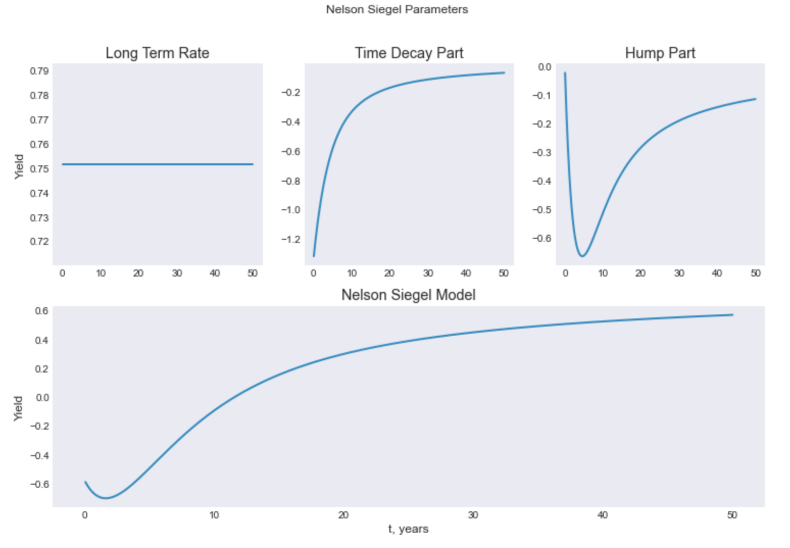
ns.plot_model()

| Attributes | Type | Description |
|---|---|---|
| beta0 | Private | Model Coefficient Beta0 |
| beta1 | Private | Model Coefficient Beta1 |
| beta2 | Private | Model Coefficient Beta2 |
| beta3 | Private | Model Coefficient Beta3 |
| tau | Private | Model Coefficient tau |
| tau2 | Private | Model Coefficient tau2 |
| attr_list | Private | Coefficient list |
| Methods | Type | Description & Params | Return |
|---|---|---|---|
| get_attr(str(attr)) | Public | attributes getter | attribute |
| set_attr(attr) | Public | attributes setter | None |
| print_model() | Public | print the Ns model set | None |
| _calibration_func(x,curve) | Private | Private method used for calibration method | float:sqr_err |
| _is_positive_attr(attr) | Private | Check attributes positivity (beta0 and tau | attribute |
| _is_valid_curve(curve) | Private | Check if the curve given for calibration is a Curve Object | Curve |
| _print_fitting() | Private | Print the result after the calibration | None |
| calibrate(curve) | Public | Minimize _calibration_func(x,curve) | sco.OptimizeResult |
| _time_decay(t) | Private | Compute the time decay part of the model t (float or array) | float,array |
| _hump(t) | Private | Compute the hump part of the model given t (float or array) | float,array |
| _second_hump(t) | Private | Compute the second hump part of the model given t (float or array) | float,array |
| d_rate(t) | Public | Get d_rate from the model for a given time t (float or array) | float,array |
| plot_calibrated() | Public | Plot Model curve against Curve | None |
| plot_model_params() | Public | Plot Model parameters | None |
| plot_model() | Public | Plot Model Components | None |
| df_t(t) | Public | Get the discount factor from the model for a given time t (float or array) | float,array |
| cdf_t(t) | Public | Get the continuous df from the model for a given time t (float or array) | float,array |
| forward_rate(t1,t2) | Public | Get the forward d_rate for a given time t1,t2 (float or array) | float,array |
Creation of a model and calibration
from PyCurve.svensson_nelson_siegel import NelsonSiegelAugmented
nss = NelsonSiegelAugmented(0.3,0.4,12,12,1,1)
nss.calibrate(curve)
Augmented Nelson Siegel Model
============================
beta0 = 0.7515069899513361
beta1 = -1.3304984652740972
beta2 = -1.3582175270153745
beta3 = -0.8621237370245594
tau = 2.5492666085730384
tau2 = 2.5493745447283485
____________________________
============================
Calibration Results
============================
CONVERGENCE: NORM_OF_PROJECTED_GRADIENT_<=_PGTOL
Mean Squared Error 0.004236730702075479
Number of Iterations 31
____________________________
Out[31]:
      fun: 0.004236730702075479
 hess_inv: <6x6 LbfgsInvHessProduct with dtype=float64>
      jac: array([-8.70041881e-06, -3.48375844e-06, -1.71824361e-06, -1.71911096e-06,
        1.00535900e-06,  3.23178986e-07])
  message: 'CONVERGENCE: NORM_OF_PROJECTED_GRADIENT_<=_PGTOL'
     nfev: 245
      nit: 31
     njev: 35
   status: 0
  success: True
        x: array([ 0.75150699, -1.33049847, -1.35821753, -0.86212374,  2.54926661,
        2.54937454])
Plotting possibilities are the same as for the Nelson-Siegel model for example
nss.plot_model_params()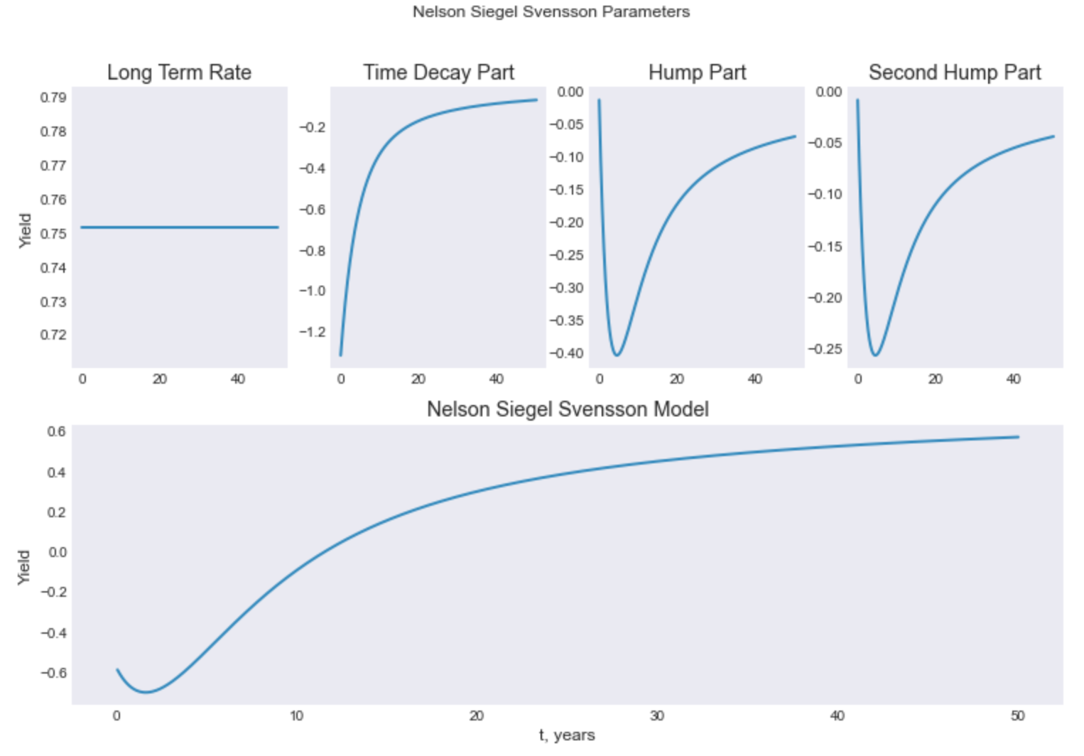
| Attributes | Type | Description |
|---|---|---|
| beta0 | Private | Model Coefficient Beta0 |
| beta1 | Private | Model Coefficient Beta1 |
| beta2 | Private | Model Coefficient Beta2 |
| beta3 | Private | Model Coefficient Beta3 |
| tau | Private | Model Coefficient tau |
| attr_list | Private | Coefficient list |
| Methods | Type | Description & Params | Return |
|---|---|---|---|
| get_attr(str(attr)) | Public | attributes getter | attribute |
| set_attr(attr) | Public | attributes setter | None |
| print_model() | Public | print the Ns model set | None |
| _calibration_func(x,curve) | Private | Private method used for calibration method | float:sqr_err |
| _is_positive_attr(attr) | Private | Check attributes positivity (beta0 and tau | attribute |
| _is_valid_curve(curve) | Private | Check if the curve given for calibration is a Curve Object | Curve |
| _print_fitting() | Private | Print the result after the calibration | None |
| calibrate(curve) | Public | Minimize _calibration_func(x,curve) | sco.OptimizeResult |
| _time_decay(t) | Private | Compute the time decay part of the model t (float or array) | float,array |
| _hump(t) | Private | Compute the hump part of the model given t (float or array) | float,array |
| _second_hump(t) | Private | Compute the second hump part of the model given t (float or array) | float,array |
| d_rate(t) | Public | Get d_rate from the model for a given time t (float or array) | float,array |
| plot_calibrated() | Public | Plot Model curve against Curve | None |
| plot_model_params() | Public | Plot Model parameters | None |
| plot_model() | Public | Plot Model Components | None |
| df_t(t) | Public | Get the discount factor from the model for a given time t (float or array) | float,array |
| cdf_t(t) | Public | Get the continuous df from the model for a given time t (float or array) | float,array |
| forward_rate(t1,t2) | Public | Get the forward d_rate for a given time t1,t2 (float or array) | float,array |
Creation of a model and calibration
from PyCurve.bjork_christensen import BjorkChristensen
bjc = BjorkChristensen(0.3,0.4,12,12,1)
bjc.calibrate(curve)
Bjork & Christensen Model
============================
beta0 = 0.7241026361747042
beta1 = 1.2630412759302045
beta2 = -4.075775255903699
beta3 = -2.61578890758314
tau = 2.0454907238894267
____________________________
============================
Calibration Results
============================
CONVERGENCE: NORM_OF_PROJECTED_GRADIENT_<=_PGTOL
Mean Squared Error 0.002575936865445517
Number of Iterations 37
____________________________
Out[36]:
      fun: 0.002575936865445517
 hess_inv: <5x5 LbfgsInvHessProduct with dtype=float64>
      jac: array([-1.34584183e-06,  7.22165387e-07, -9.63335320e-07,  1.34501786e-06,
        4.57750160e-07])
  message: 'CONVERGENCE: NORM_OF_PROJECTED_GRADIENT_<=_PGTOL'
     nfev: 252
      nit: 37
     njev: 42
   status: 0
  success: True
        x: array([ 0.72410264,  1.26304128, -4.07577526, -2.61578891,  2.04549072])
Plotting possibilities are the same as for the Nelson-Siegel model for example
bjc.plot_model()
| Attributes | Type | Description |
|---|---|---|
| beta0 | Private | Model Coefficient Beta0 |
| beta1 | Private | Model Coefficient Beta1 |
| beta2 | Private | Model Coefficient Beta2 |
| beta3 | Private | Model Coefficient Beta3 |
| beta4 | Private | Model Coefficient Beta4 |
| tau | Private | Model Coefficient tau |
| attr_list | Private | Coefficient list |
| Methods | Type | Description & Params | Return |
|---|---|---|---|
| get_attr(str(attr)) | Public | attributes getter | attribute |
| set_attr(attr) | Public | attributes setter | None |
| print_model() | Public | print the Ns model set | None |
| _calibration_func(x,curve) | Private | Private method used for calibration method | float:sqr_err |
| _is_positive_attr(attr) | Private | Check attributes positivity (beta0 and tau | attribute |
| _is_valid_curve(curve) | Private | Check if the curve given for calibration is a Curve Object | Curve |
| _print_fitting() | Private | Print the result after the calibration | None |
| calibrate(curve) | Public | Minimize _calibration_func(x,curve) | sco.OptimizeResult |
| _time_decay(t) | Private | Compute the time decay part of the model t (float or array) | float,array |
| _hump(t) | Private | Compute the hump part of the model given t (float or array) | float,array |
| _second_hump(t) | Private | Compute the second hump part of the model given t (float or array) | float,array |
| _third_hump(t) | Private | Compute the third hump part of the model given t (float or array) | float,array |
| d_rate(t) | Public | Get d_rate from the model for a given time t (float or array) | float,array |
| plot_calibrated() | Public | Plot Model curve against Curve | None |
| plot_model_params() | Public | Plot Model parameters | None |
| plot_model() | Public | Plot Model Components | None |
| df_t(t) | Public | Get the discount factor from the model for a given time t (float or array) | float,array |
| cdf_t(t) | Public | Get the continuous df from the model for a given time t (float or array) | float,array |
| forward_rate(t1,t2) | Public | Get the forward d_rate for a given time t1,t2 (float or array) | float,array |
Creation of a model and calibration
from PyCurve.bjork_christensen_augmented import BjorkChristensenAugmented
bjc_a = BjorkChristensenAugmented(0.3,0.4,12,12,12,1)
bjc_a.calibrate(curve)
Bjork & Christensen Augmented Model
============================
beta0 = 1.5954945516202643
beta1 = -0.1362673420894012
beta2 = -1.921347491829477
beta3 = -3.100138400789165
beta4 = -0.2790540854856497
tau = 3.3831338085688625
____________________________
============================
Calibration Results
============================
CONVERGENCE: REL_REDUCTION_OF_F_<=_FACTR*EPSMCH
Mean Squared Error 4.6222147406189135e-05
Number of Iterations 45
____________________________
Out[39]:
      fun: 4.6222147406189135e-05
 hess_inv: <6x6 LbfgsInvHessProduct with dtype=float64>
      jac: array([-3.13922277e-05, -1.14224797e-04, -3.47444433e-05,  2.07803821e-05,
        7.91378953e-06,  6.50288949e-06])
  message: 'CONVERGENCE: REL_REDUCTION_OF_F_<=_FACTR*EPSMCH'
     nfev: 357
      nit: 45
     njev: 51
   status: 0
  success: True
        x: array([ 1.59549455, -0.13626734, -1.92134749, -3.1001384 , -0.27905409,
        3.38313381])
Plotting possibilities are the same as for the Nelson-Siegel model for example
bjc_a.plot_calibrated(curve)
| Attributes | Type | Description |
|---|---|---|
| alpha | Private | Model Coefficient alpha (mean reverting speed) |
| beta | Private | Model Coefficient Beta (long term mean) |
| sigma | Private | Short rate Volatility |
| rt | Private | Initial Short Rate |
| time | Params | Time in years |
| dt | Private | time for each period |
| steps | Private | calculated with dt & time as time/dt |
| Methods | Type | Description & Params | Return |
|---|---|---|---|
| get_attr(str(attr)) | Public | attributes getter | attribute |
| sigma_part(n) | Private | compute n sigma part | float |
| mu_dt(rt) | Private | compute drift part | float |
| simulate_paths(n) | Public | Simulate n Short rate paths | np.ndarray |
| plot_calibrated(simul,curve) | Public | Plot yield curve against simulate curve | None |
time = np.array([0.25, 0.5, 0.75, 1., 2.,
                 3., 4., 5., 10., 15.,
                 20., 25., 30.])
rate = np.array([-0.0063171, -0.00650322, -0.00664493, -0.00674608, -0.00681294,
                 -0.00647593, -0.00587828, -0.0051251, -0.00101804, 0.00182851,
                 0.0032962, 0.0030092117, 0.00412151])
curve = Curve(time,rate)
vasicek_model = Vasicek(0.5, 0.0040, 0.001, -0.0067, 30, 1 / 365)
simulation = vasicek_model.simulate_paths(200)
vasicek_model.plot_calibrated(simulation,curve)
All the tools for graphing from simulation could be applied to vasicek simulation results.

| Attributes | Type | Description |
|---|---|---|
| alpha | Private | Model Coefficient alpha (mean reverting speed) |
| sigma | Private | Short rate Volatility |
| rt | Private | Initial Short Rate |
| time | Params | Time in years |
| dt | Private | time for each period |
| steps | Private | calculated with dt & time as time/dt |
| f_curve | Private | Curve : Initial instantaneous forward structure |
| method | Private | method used in order to interpolate f_curve |
| Methods | Type | Description & Params | Return |
|---|---|---|---|
| get_attr(str(attr)) | Public | attributes getter | attribute |
| _is_valid_curve(curve) | Private | Check if the curve given for calibration is a Curve Object | Curve |
| sigma_part(n) | Private | compute n sigma part | float |
| interp_forward(t) | Private | interpolate forward curve for maturity t | float |
| theta_part(t) | Private | compute theta(t) | float |
| mu_dt(rt,t) | Private | compute drift part at time t | float |
| simulate_paths(n) | Public | Simulate n Short rate paths | np.ndarray |
| plot_calibrated(simul) | Public | Plot yield curve against simulate curve | None |
from PyCurve.bjork_christensen_augmented import BjorkChristensenAugmented
from PyCurve.hull_white import HullWhite
import numpy as np
from PyCurve.curve import Curve
# Instance of curve : Spot Rates
time = np.array([0.25, 0.5, 0.75, 1., 2.,
3., 4., 5., 10., 15.,
20., 25., 30.])
rate = np.array([-0.0063171, -0.00650322, -0.00664493, -0.00674608, -0.00681294,
-0.00647593, -0.00587828, -0.0051251, -0.00101804, 0.00182851,
0.0032962, 0.00392117, 0.00412151])
curve = Curve(time, rate)
# Deduce Forward rate via Bjork Christensen (as example but you can directly create an instance of Curve with values)
bjc_a = BjorkChristensenAugmented(0.3, 0.4, 12, 12, 12, 1)
bjc_a.calibrate(curve)
forward_curve = [-0.006301821217413436379]
forward_curve_t = [0]
for i in range(12):
forward_curve.append(bjc_a.forward_rate(time[i], time[i + 1]))
forward_curve_t.append(time[i])
instantaneous_forward = Curve(forward_curve_t, forward_curve)
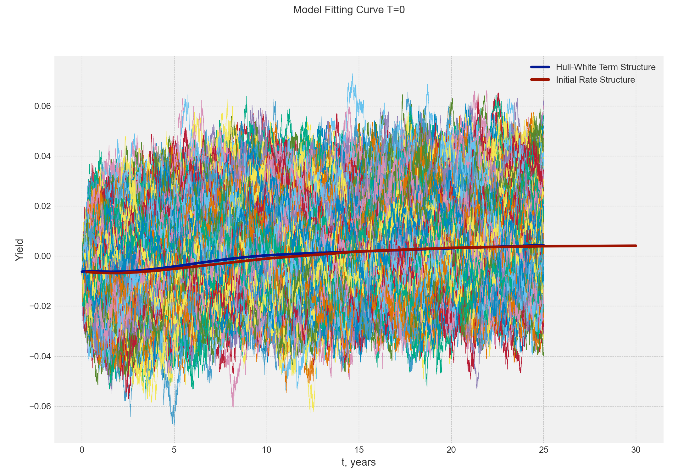
# Hull and white model with High Volatility
hull_white_model = HullWhite(1, 0.02, -0.0063, 25, 1 / 365, instantaneous_forward, 'linear')
simulation = hull_white_model.simulate_paths(1000)
hull_white_model.plot_calibrated(simulation,curve)
Bjork & Christensen Augmented Model
============================
beta0 = 0.0003242320890548229
beta1 = 0.00042283628067360974
beta2 = 0.014729859086888815
beta3 = -0.03083749691652102
beta4 = -0.020626731632810553
tau = 1.137911384276111
____________________________
============================
Calibration Results
============================
CONVERGENCE: REL_REDUCTION_OF_F_<=_FACTR*EPSMCH
Mean Squared Error 3.084012924460394e-06
Number of Iterations 24
____________________________
All the tools for graphing from simulation could be applied to Hull-White simulation results.
# Hull and white model  with High Volatility
hull_white_model_low_vol = HullWhite(1, 0.00002, -0.0063, 25, 1 / 365, instantaneous_forward, 'cubic')
simulation = hull_white_model_low_vol.simulate_paths(1000)
simulation.plot_model()
hull_white_model_low_vol.plot_calibrated(simulation,curve)


